Sliced Australia Weather

workflowr

• Summary
• Checks
• Past versions

Last updated: 2021-10-10

Checks: 7 0

Knit directory: myTidyTuesday/

This reproducible R Markdown analysis was created with workflowr (version 1.6.2). The Checks tab describes the reproducibility checks that were applied when the results were created. The Past versions tab lists the development history.

---

R Markdown file: up-to-date

Great! Since the R Markdown file has been committed to the Git repository, you know the exact version of the code that produced these results.

Environment: empty

Great job! The global environment was empty. Objects defined in the global environment can affect the analysis in your R Markdown file in unknown ways. For reproduciblity it’s best to always run the code in an empty environment.

Seed: set.seed(20210907)

The command set.seed(20210907) was run prior to running the code in the R Markdown file. Setting a seed ensures that any results that rely on randomness, e.g. subsampling or permutations, are reproducible.

Session information: recorded

Great job! Recording the operating system, R version, and package versions is critical for reproducibility.

Cache: none

Nice! There were no cached chunks for this analysis, so you can be confident that you successfully produced the results during this run.

File paths: relative

Great job! Using relative paths to the files within your workflowr project makes it easier to run your code on other machines.

Repository version: e42de19

Great! You are using Git for version control. Tracking code development and connecting the code version to the results is critical for reproducibility.

The results in this page were generated with repository version e42de19. See the Past versions tab to see a history of the changes made to the R Markdown and HTML files.

Note that you need to be careful to ensure that all relevant files for the analysis have been committed to Git prior to generating the results (you can use wflow_publish or wflow_git_commit). workflowr only checks the R Markdown file, but you know if there are other scripts or data files that it depends on. Below is the status of the Git repository when the results were generated:

Ignored files:
    Ignored:    .Rhistory
    Ignored:    .Rproj.user/
    Ignored:    catboost_info/
    Ignored:    data/2021-09-08/
    Ignored:    data/2021-10-10/
    Ignored:    data/CNHI_Excel_Chart.xlsx
    Ignored:    data/CommunityTreemap.jpeg
    Ignored:    data/Community_Roles.jpeg
    Ignored:    data/YammerDigitalDataScienceMembership.xlsx
    Ignored:    data/acs_poverty.rds
    Ignored:    data/australiaweather.rds
    Ignored:    data/fmhpi.rds
    Ignored:    data/grainstocks.rds
    Ignored:    data/hike_data.rds
    Ignored:    data/nber_rs.rmd
    Ignored:    data/netflixTitles.rmd
    Ignored:    data/netflixTitles2.rds
    Ignored:    data/us_states.rds
    Ignored:    data/us_states_hexgrid.geojson
    Ignored:    data/weatherstats_toronto_daily.csv

Untracked files:
    Untracked:  analysis/CHN_1_sp.rds
    Untracked:  analysis/sample data for r test.xlsx
    Untracked:  code/YammerReach.R
    Untracked:  code/work list batch targets.R

Note that any generated files, e.g. HTML, png, CSS, etc., are not included in this status report because it is ok for generated content to have uncommitted changes.

---

These are the previous versions of the repository in which changes were made to the R Markdown (analysis/2021_06_22_sliced.Rmd) and HTML (docs/2021_06_22_sliced.html) files. If you’ve configured a remote Git repository (see ?wflow_git_remote), click on the hyperlinks in the table below to view the files as they were in that past version.

File	Version	Author	Date	Message
Rmd	e42de19	opus1993	2021-10-10	use new confusion matrix autoplot method

---

SLICED is like the TV Show Chopped but for data science. Competitors get a never-before-seen dataset and two-hours to code a solution to a prediction challenge. Contestants get points for the best model plus bonus points for data visualization, votes from the audience, and more.

Season 1 Episode 4 featured David Robinson, Craig Mann, Greg Matthews, and Jesse Mostipak in a challenge to predict whether it will rain tomorrow in several cities in Australia from daily data.

There are several choices of algorithmic approaches available. For example, each location city could be modeled as it’s own time series. Pooling the effects across all cities geographically would be a computational challenge this way. If we were looking for climactic shifts and large weather patterns, it might be worth the time. But we only have 2 hours.

In a real-world project, we would map out the costs of correct and incorrect predictions, model for ROC (area under the curve), and then adjust the cutoff value for sensitivity and specificity (ratios of false positive rates and false negative rates). The evaluation metric in this competition is simply to minimize the mean LogLoss values of the probabilities of the classifier.

To make the best use of the resources that we have, we will explore the data set features to select those with the most predictive power, build and tune several fast GLMnet regularized models to confirm the receipe, and then use the rest of the time to build one or more XGBoost ensemble models. If we have time, we will stack several of the

Let’s load up some packages:

suppressPackageStartupMessages({
library(tidyverse)
library(hrbrthemes)
library(lubridate)
  
library(tidymodels)
library(textrecipes)
library(treesnip)
library(finetune)
library(stacks)
library(themis)
  
library(tidycensus)
options(tigris_use_cache = TRUE)

library(patchwork)
})

source(here::here("code","_common.R"),
       verbose = FALSE,
       local = knitr::knit_global())

ggplot2::theme_set(theme_jim(base_size = 12))

#create a data directory
data_dir <- here::here("data",Sys.Date())
if (!file.exists(data_dir)) dir.create(data_dir)

# set a competition metric
mset <- metric_set(mn_log_loss)

# set the competition name from the web address
competition_name <- "sliced-s01e04-knyna9"

zipfile <- paste0(data_dir,"/", competition_name, ".zip")

path_export <- here::here("data",Sys.Date(),paste0(competition_name,".csv"))

A quick reminder before downloading the dataset: Go to the web site and accept the competition terms!!!

Import and EDA

Unlike the contestants, I built a template hoping to get a jump on model building when the dataset became available. I learned that my approach needs more work to finish within 2 hours. I am impressed with the skills of the contestants.

This file is the result of a full day of reflecting on my mistakes and includes some of the best parts of what the contestants demonstrated, live coding from scratch.

Direct Import and Skim

We have basic shell commands available to interact with Kaggle here:

# from the Kaggle api https://github.com/Kaggle/kaggle-api

# the leaderboard
shell(glue::glue("kaggle competitions leaderboard { competition_name } -s"))

# the files to download
shell(glue::glue("kaggle competitions files -c { competition_name }"))

# the command to download files
shell(glue::glue("kaggle competitions download -c { competition_name } -p { data_dir }"))

# unzip the files received
shell(glue::glue("unzip { zipfile } -d { data_dir }"))

Reading in the contents of the datafiles here:

train_df <- read_csv(file = glue::glue(
  {
    data_dir
  },
  "/train.csv"
)) %>%
  mutate_if(is.character, as.factor) %>%
  mutate(
    rain_tomorrow = as.factor(rain_tomorrow),
    rain_today = as.factor(rain_today)
  )

test_df <- read_csv(file = glue::glue(
  {
    data_dir
  },
  "/test.csv"
)) %>%
  mutate_if(is.character, as.factor) %>%
  mutate(rain_today = as.factor(rain_today))

Some questions to answer here: What features have missing data, and imputations may be required? What does the outcome variable look like, in terms of imbalance?

skimr::skim(train_df)

Feature plots

Let’s explore the relationships between the features and the rainfall likelihood. First, let’s build a function to summarize the counts of rainfall days and the ratio of rainfall days within a grouping.

summarize_rainfall <- function(tbl) {
  ret <- tbl %>%
    summarize(
      n_rain = sum(rain_tomorrow == 1),
      n = n(),
      .groups = "drop"
    ) %>%
    arrange(desc(n)) %>%
    mutate(
      pct_rain = n_rain / n,
      low = qbeta(.025, n_rain + 5, n - n_rain + .5),
      high = qbeta(.975, n_rain + 5, n - n_rain + .5)
    ) %>%
    mutate(pct = n / sum(n))
  ret
}

train_df %>%
  summarize_rainfall()

train_df %>%
  group_by(location = fct_lump(location, 30)) %>%
  summarize_rainfall() %>%
  mutate(location = fct_reorder(location, pct_rain)) %>%
  ggplot(aes(pct_rain, location)) +
  geom_point(aes(size = pct)) +
  geom_errorbarh(aes(xmin = low, xmax = high), height = .3) +
  scale_size_continuous(
    labels = percent,
    guide = "none",
    range = c(.5, 4)
  ) +
  scale_x_continuous(labels = percent_format(accuracy = 1)) +
  labs(
    x = "Probability of raining tomorrow",
    y = "",
    title = "What locations get the most rain?",
    subtitle = "Including 95% confidence intervals. Size of points is proportional to frequency"
  ) +
  theme(panel.grid.major.y = element_blank())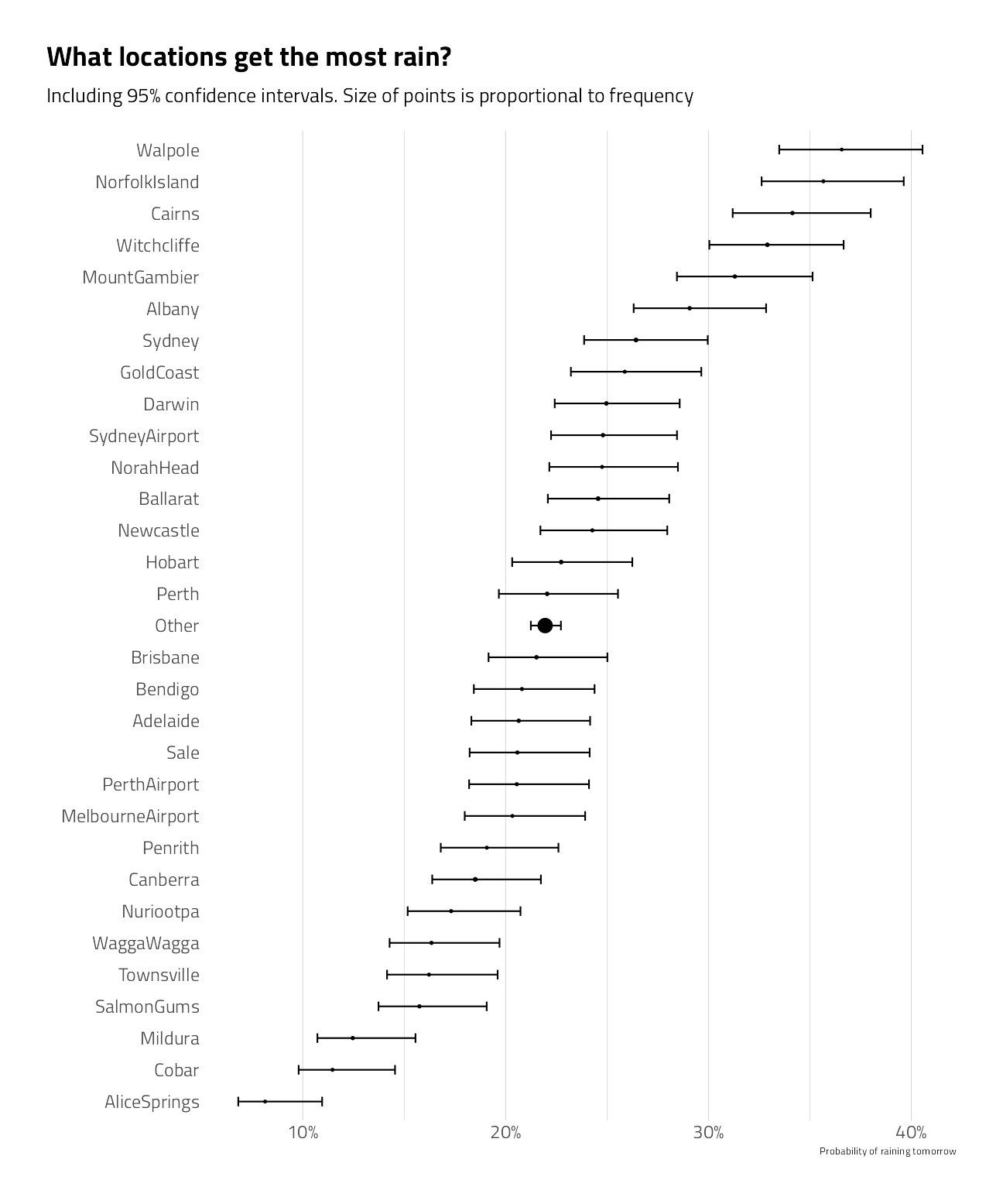

A plot of the time series by year and the range within the year

train_df %>%
  group_by(year = year(date)) %>%
  summarize_rainfall() %>%
  ggplot(aes(year, pct_rain)) +
  geom_point(aes(size = n)) +
  geom_line() +
  geom_ribbon(aes(ymin = low, ymax = high), alpha = .1) +
  expand_limits(y = 0) +
  scale_x_continuous(breaks = seq(2007, 2017, 2)) +
  scale_y_continuous(labels = percent_format()) +
  scale_size_continuous(guide = "none") +
  coord_cartesian(ylim = c(0, .35)) +
  labs(
    x = "Year", y = NULL,
    title = "% days rain tomorrow in each year"
  )

train_numeric <- train_df %>%
  keep(is.numeric) %>%
  colnames()

chart <- c(train_numeric, "rain_tomorrow")

train_df %>%
  select_at(vars(all_of(chart))) %>%
  select(-id) %>%
  pivot_longer(
    cols = c(
      min_temp,
      max_temp,
      rainfall,
      contains("speed"),
      contains("humidity"),
      contains("pressure"),
      contains("cloud"),
      contains("temp")
    ),
    names_to = "key",
    values_to = "value"
  ) %>%
  filter(!is.na(value)) %>%
  ggplot() +
  geom_histogram(
    mapping = aes(
      x = value,
      fill = rain_tomorrow
    ),
    bins = 50,
    show.legend = FALSE
  ) +
  facet_wrap(~key,
    scales = "free",
    ncol = 4
  ) +
  scale_x_continuous(n.breaks = 3) +
  scale_y_continuous(n.breaks = 3) +
  theme(
    plot.subtitle = ggtext::element_textbox_simple(),
    plot.background = element_rect(color = "white")
  ) +
  labs(
    title = "Numeric Feature Histogram Distributions",
    subtitle = "<span style = 'color:#F1CA3AFF'>Rainy days</span> and <span style = 'color:#7A0403FF'> not rainy days</span>",
    x = NULL, y = NULL
  )

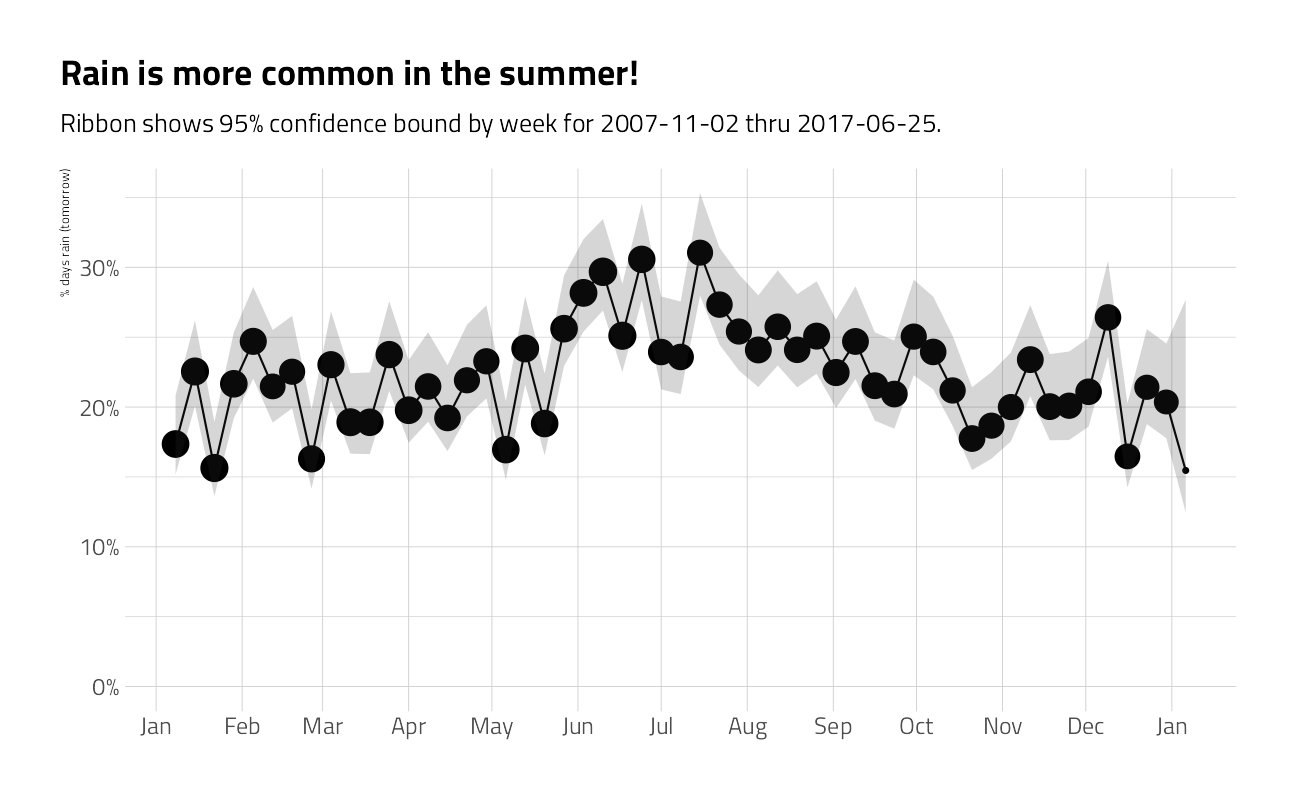
train_df %>%
  group_by(week = as.Date("2020-01-01") + week(date) * 7) %>%
  summarize_rainfall() %>%
  ggplot(aes(week, pct_rain)) +
  geom_point(aes(size = n)) +
  geom_line() +
  geom_ribbon(aes(ymin = low, ymax = high), alpha = .2) +
  expand_limits(y = 0) +
  scale_x_date(
    date_labels = "%b",
    date_breaks = "month",
    minor_breaks = NULL
  ) +
  scale_y_continuous(labels = percent) +
  scale_size_continuous(guide = "none") +
  labs(
    x = NULL,
    y = "% days rain (tomorrow)",
    title = "Rain is more common in the summer!",
    subtitle = glue::glue("Ribbon shows 95% confidence bound by week for { min(train_df$date) } thru { max(train_df$date) }.")
  )

David Robinson’s beautiful compass rose

compass_directions <- c(
  "N", "NNE", "NE", "ENE", "E", "ESE", "SE", "SSE", "S",
  "SSW", "SW", "WSW", "W", "WNW", "NW", "NNW"
)
as_angle <- function(direction) {
  (match(direction, compass_directions) - 1) * 360 / length(compass_directions)
}

train_df %>%
  pivot_longer(
    cols = contains("dir"),
    names_to = "type",
    values_to = "direction"
  ) %>%
  mutate(
    type = str_remove(type, "wind_dir"),
    type = ifelse(type == "wind_gust_dir", "Overall", type)
  ) %>%
  group_by(type, direction) %>%
  summarize_rainfall() %>%
  filter(!is.na(direction)) %>%
  mutate(angle = as_angle(direction)) %>%
  ggplot(aes(angle)) +
  geom_line(aes(y = pct_rain, color = type),
    show.legend = FALSE
  ) +
  geom_text(aes(y = .35, label = direction),
    size = 6, hjust = 0.5
  ) +
  annotate("text",
    x = 120,
    y = c(0, 0.1, 0.2, 0.3),
    label = c(0, 10, 20, 30),
    size = 3
  ) +
  scale_y_continuous(labels = percent) +
  expand_limits(x = c(0, 360), y = 0) +
  coord_polar(start = 0, theta = "x", ) +
  labs(
    x = NULL,
    y = "% when wind is in this direction",
    title = "Rain tomorrow depends upon the compass direction",
    subtitle = "<span style = 'color:#F1CA3AFF'>3pm </span>, <span style = 'color:#7A0403FF'> 9am</span>, and <span style = 'color:#1FC8DEFF'> Overall</span>",
    color = "Time"
  ) +
  theme(
    plot.subtitle = ggtext::element_textbox_simple(),
    panel.grid.minor.x = element_blank(),
    panel.grid.major.x = element_blank()
  )

Looking for interaction terms in change over day!

spread_time <- train_df %>%
  select(id, rain_tomorrow, contains("3"), contains("9")) %>%
  select(-contains("dir")) %>%
  pivot_longer(
    cols = c(-rain_tomorrow, -id),
    names_to = "metric",
    values_to = "value"
  ) %>%
  separate(metric, c("metric", "time"), sep = -3) %>%
  mutate(time = paste0("at_", time)) %>%
  filter(!is.na(value)) %>%
  pivot_wider(
    names_from = "time",
    values_from = "value"
  )

spread_time %>%
  filter(!is.na(at_9am), !is.na(at_3pm)) %>%
  ggplot(aes(at_9am, at_3pm)) +
  geom_point(shape = 21, alpha = 0.1) +
  geom_smooth(aes(color = rain_tomorrow),
    method = "lm",
    formula = "y ~ x",
    show.legend = FALSE
  ) +
  facet_wrap(~metric, scales = "free") +
  theme(plot.subtitle = ggtext::element_textbox_simple()) +
  labs(
    x = "9 AM",
    y = "3 PM",
    title = "Does the difference in time of day change rain/won't rain?",
    subtitle = "<span style = 'color:#F1CA3AFF'>Rainy days</span> and <span style = 'color:#7A0403FF'> not rainy days</span>",
    color = ""
  )

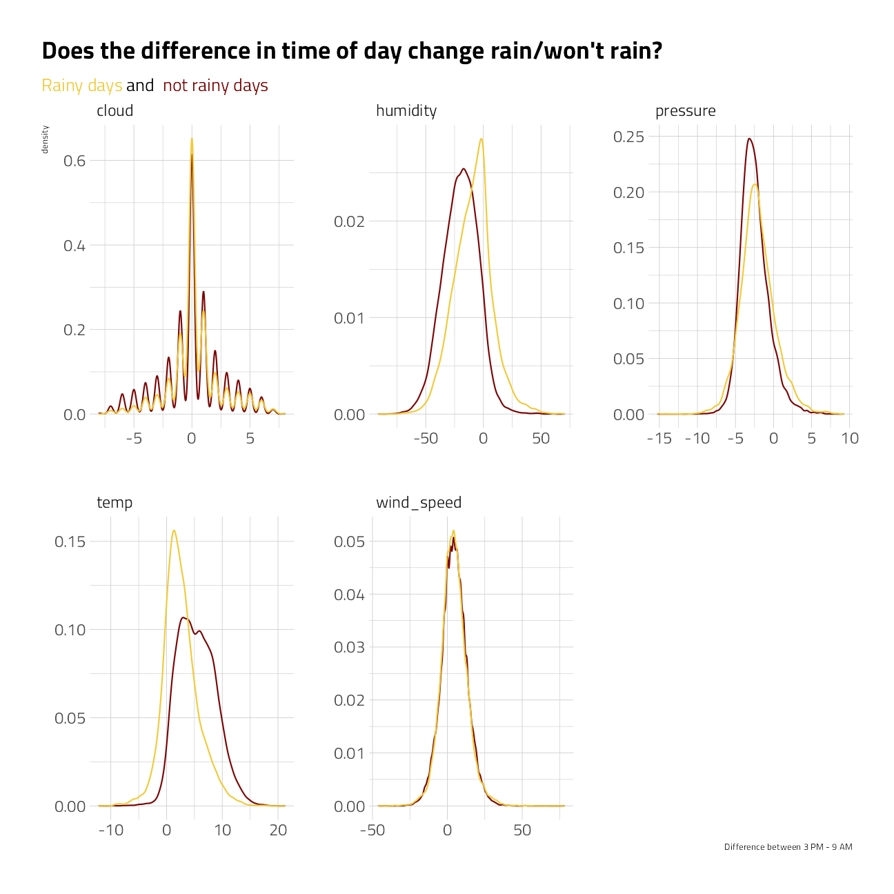
spread_time %>%
  filter(!is.na(at_9am), !is.na(at_3pm)) %>%
  ggplot(aes(at_3pm - at_9am)) +
  geom_density(aes(color = rain_tomorrow), show.legend = FALSE) +
  facet_wrap(~metric, scales = "free") +
  theme(plot.subtitle = ggtext::element_textbox_simple()) +
  labs(
    x = "Difference between 3 PM - 9 AM",
    title = "Does the difference in time of day change rain/won't rain?",
    subtitle = "<span style = 'color:#F1CA3AFF'>Rainy days</span> and <span style = 'color:#7A0403FF'> not rainy days</span>",
    color = NULL, fill = NULL
  )

Numeric Feature Correlations

cr1 <- train_df %>%
  select(-id) %>%
  keep(is.numeric) %>%
  cor(use = "pair")

corrplot::corrplot(cr1, type = "upper")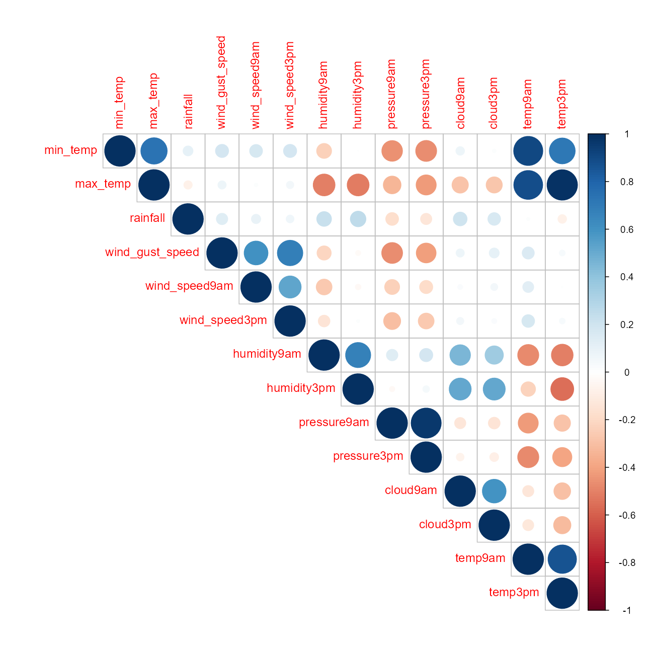

Conclusions:

• If humidity increased between 9am and 3pm, likely to rain
• If temp increased between 9am and 3pm, less likely to rain
• If cloud cover increased between 9am and 3pm, more likely to rain
• Little effect of change in wind speed or pressure from 9am to 3pm

Preprocessiong

The recipe framework

I am going to train on almost all of the train data. The 1% left is a quick confirmation of validity. The provided file labeled test has no labels.

set.seed(2021)
split <- initial_split(train_df,
  strata = rain_tomorrow,
  prop = .99
)
train <- training(split)
valid <- testing(split)

There are only 343 held out from training as a last check before submission.

rec <-
  recipe(rain_tomorrow ~ ., train) %>%
  # ---- set aside the row id's
  update_role(id, new_role = "id") %>%
  step_date(date,
    features = c("doy", "year"),
    keep_original_cols = FALSE
  ) %>%
  step_rm(evaporation, sunshine) %>%
  step_log(rainfall, offset = 1, base = 2) %>%
  step_impute_median(all_numeric_predictors()) %>%
  step_ns(date_doy, deg_free = 4) %>%
  step_ns(date_year, deg_free = 2) %>%
  step_mutate(wind_gust_dir = str_sub(wind_gust_dir, 1, 1)) %>%
  step_mutate(wind_dir9am = str_sub(wind_dir9am, 1, 1)) %>%
  step_mutate(wind_dir3pm = str_sub(wind_dir3pm, 1, 1)) %>%
  step_mutate(
    cloud9am = if_else(is.na(cloud9am),
      0, cloud9am
    ),
    cloud3pm = if_else(is.na(cloud3pm),
      0, cloud3pm
    ),
    cloud_change = cloud3pm - cloud9am
  ) %>%
  step_rm(cloud9am, cloud3pm) %>%
  step_mutate(
    humidity9am = if_else(is.na(humidity9am),
      0, humidity9am
    ),
    humidity3pm = if_else(is.na(humidity3pm),
      0, humidity3pm
    ),
    humidity_change = humidity3pm - humidity9am
  ) %>%
  step_rm(humidity9am, humidity3pm) %>%
  step_novel(all_nominal_predictors()) %>%
  step_unknown(all_nominal_predictors()) %>%
  step_dummy(all_nominal_predictors()) %>%
  step_upsample(rain_tomorrow)

the pre-processed data

rec %>%
  #  finalize_recipe(list(num_comp = 2)) %>%
  prep() %>%
  juice()

Cross Validation

We will use 5-fold cross validation and stratify between the rain and no-rain classes.

train_folds <- vfold_cv(
  data = train,
  strata = rain_tomorrow,
  v = 5
)

ggplot(
  train_folds %>% tidy(),
  aes(Fold, Row, fill = Data)
) +
  geom_tile() +
  labs(caption = "Resampling strategy")

Machine Learning

Model Specifications

We will build a specification for regularized logistic regression as GLMnet and a specification for XGboost.

# see parsnip::parsnip_addin()
xgboost_spec <- boost_tree(
  mtry = tune(),
  trees = tune(),
  min_n = tune(),
  tree_depth = tune(),
  learn_rate = .01
) %>%
  set_engine("xgboost") %>%
  set_mode("classification")

glmnet_spec <-
  logistic_reg(penalty = tune(), mixture = tune()) %>%
  set_engine("glmnet") %>%
  set_mode("classification")

Parallel backend

To speed up computation we will use a parallel backend.

all_cores <- parallelly::availableCores(omit = 1)
future::plan("multisession", workers = all_cores) # on Windows

Tuning GLMnet

Let’s look each modeling technique individually, glmnet first. With so many predictors, I expect to see some drop out.

cv_res_glm <-
  workflow() %>%
  add_recipe(rec) %>%
  add_model(glmnet_spec) %>%
  tune_grid(
    resamples = train_folds,
    control = control_stack_resamples(),
    grid = crossing(
      penalty = 10^seq(-7, -1, 1),
      mixture = 0.1
    ),
    metrics = mset
  )

autoplot(cv_res_glm)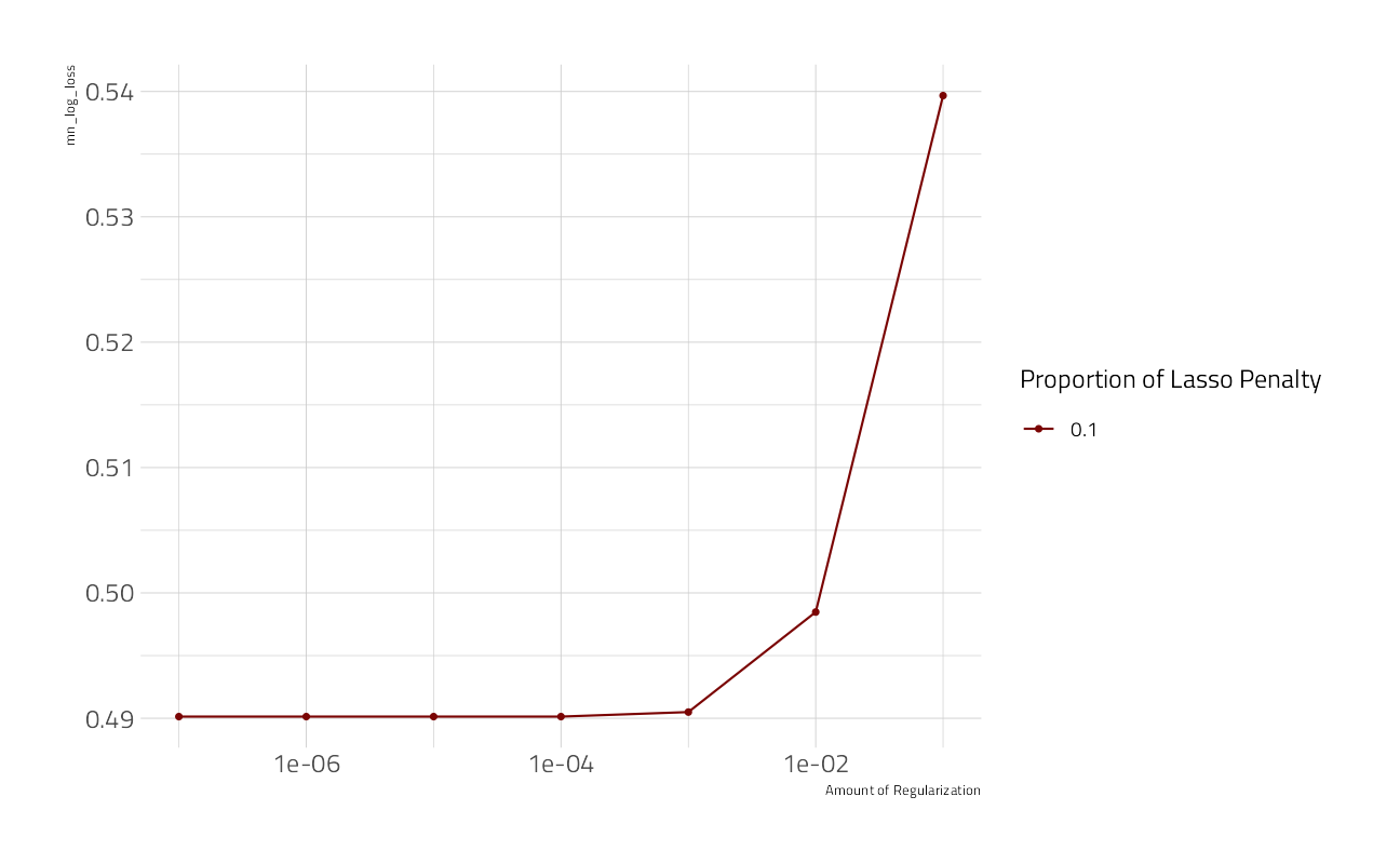

show_best(cv_res_glm) %>%
  select(-.estimator)

When mixture = 1 the glmnet model regularization is pure lasso, without any ridge terms.

What feature coefficients does the lasso keep?

workflow() %>%
  add_recipe(rec) %>%
  add_model(glmnet_spec) %>%
  finalize_workflow(select_best(cv_res_glm)) %>%
  fit(train) %>%
  extract_fit_engine() %>%
  tidy() %>%
  filter(!str_detect(term, "Intercept")) %>%
  ggplot() +
  geom_line(aes(lambda, estimate, color = term),
    show.legend = FALSE
  ) +
  scale_x_log10() +
  geom_vline(xintercept = select_best(cv_res_glm)$penalty) +
  annotate("text",
    hjust = 0,
    x = select_best(cv_res_glm)$penalty,
    y = 1,
    label = "Optimal Lasso penalty"
  ) +
  labs(title = "GLMNet model retains all of the features")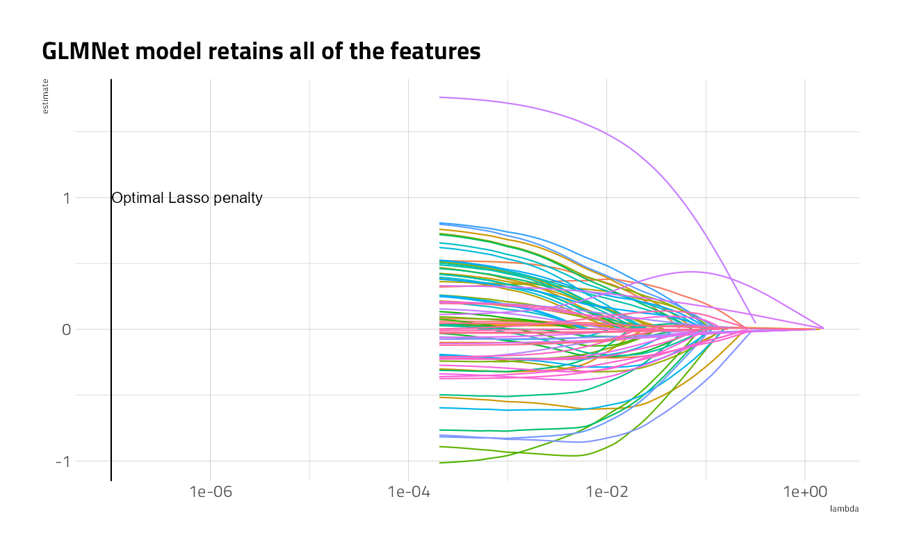

Tuning XGBoost

Now that we have some confidence that the features have predictive power, lets tune up a set of XGBoost models.

cv_res_xgboost <-
  workflow() %>%
  add_recipe(rec) %>%
  add_model(xgboost_spec) %>%
  tune_grid(
    resamples = train_folds,
    control = control_race(
      verbose_elim = TRUE,
      save_pred = TRUE,
      save_workflow = TRUE
    ),
    iter = 4,
    metrics = mset
  )

autoplot(cv_res_xgboost)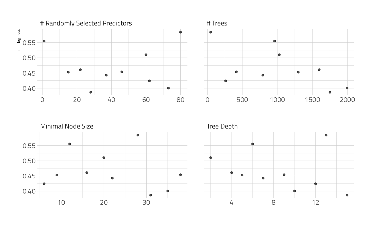

show_best(cv_res_xgboost) %>%
  select(-.estimator)

xg_wf_best <-
  workflow() %>%
  add_recipe(rec) %>%
  add_model(xgboost_spec) %>%
  finalize_workflow(select_best(cv_res_xgboost))

xg_fit_best <- xg_wf_best %>%
  fit(train)

[20:08:36] WARNING: amalgamation/../src/learner.cc:1095: Starting in XGBoost 1.3.0, the default evaluation metric used with the objective 'binary:logistic' was changed from 'error' to 'logloss'. Explicitly set eval_metric if you'd like to restore the old behavior.

vip::vip(xg_fit_best$fit$fit$fit) +
  labs("XGBoost Feature Importance")

predict(xg_fit_best, new_data = valid, type = "prob") %>%
  cbind(valid) %>%
  mn_log_loss(rain_tomorrow, `.pred_0`)

The best XGBoost model has a considerably better performance, at least on the training data.

Next steps:

• Blend linear and xgboost into an ensemble

Stack the Ensemble

The stacks package will select from all of the candidate models used in hyperparameter tuning from the GLMnet and the XGBoost sessions above and blend a weighted subset of several.

Blend the Predictions

stacked_model <- stacks() %>%
  add_candidates(cv_res_glm) %>%
  add_candidates(cv_res_xgboost) %>%
  blend_predictions()

autoplot(stacked_model, type = "weights")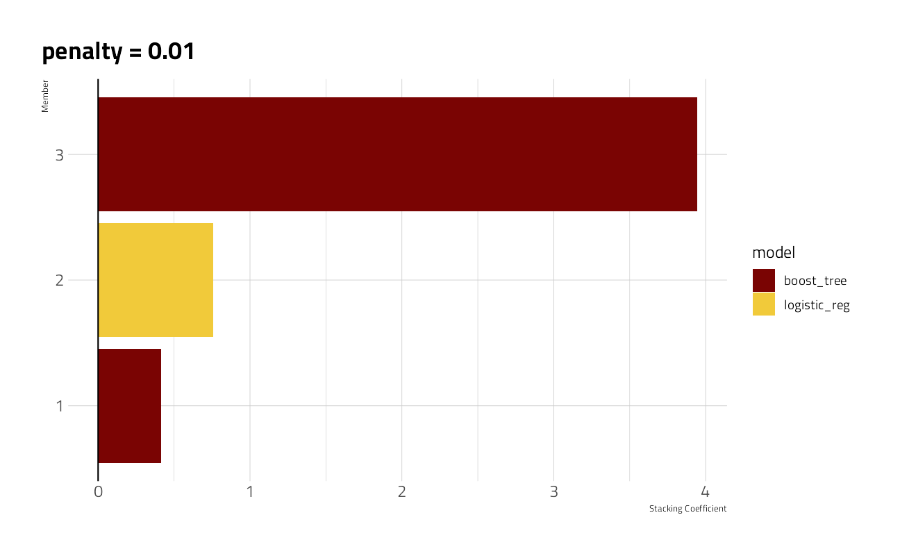

Fit the members

final_model <- stacked_model %>%
  fit_members()

[20:15:35] WARNING: amalgamation/../src/learner.cc:1095: Starting in XGBoost 1.3.0, the default evaluation metric used with the objective 'binary:logistic' was changed from 'error' to 'logloss'. Explicitly set eval_metric if you'd like to restore the old behavior.
[20:20:15] WARNING: amalgamation/../src/learner.cc:1095: Starting in XGBoost 1.3.0, the default evaluation metric used with the objective 'binary:logistic' was changed from 'error' to 'logloss'. Explicitly set eval_metric if you'd like to restore the old behavior.

A quick confirmation look at the predictions on the held out data as a confusion matrix:

bind_cols(predict(final_model, valid), valid) %>%
  yardstick::conf_mat(
    truth = rain_tomorrow,
    estimate = .pred_class
  ) %>%
  autoplot()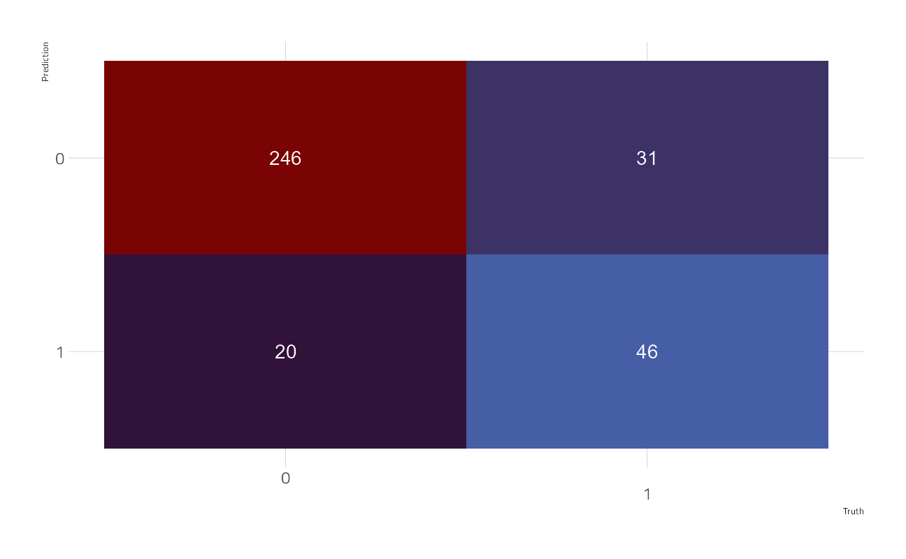

bind_cols(predict(final_model, valid, type = "prob"), valid) %>%
  yardstick::mn_log_loss(
    truth = rain_tomorrow,
    estimate = .pred_0
  )

Lastly, we build the submission file

bind_cols(predict(final_model, test_df, type = "prob"), test_df) %>%
  select(id, rain_tomorrow = .pred_0) %>%
  write_csv(file = path_export)

and make the submission to the Kaggle board

shell(glue::glue('kaggle competitions submit -c { competition_name } -f { path_export } -m "My Submission Message"'))

I am not entirely satisfied with the results. Even so, we only had two hours, and the logloss figure here is among the top rankings.

Session information

sessionInfo()

R version 4.1.1 (2021-08-10)
Platform: x86_64-w64-mingw32/x64 (64-bit)
Running under: Windows 10 x64 (build 22000)

Matrix products: default

locale:
[1] LC_COLLATE=English_United States.1252 
[2] LC_CTYPE=English_United States.1252   
[3] LC_MONETARY=English_United States.1252
[4] LC_NUMERIC=C                          
[5] LC_TIME=English_United States.1252    

attached base packages:
[1] stats     graphics  grDevices utils     datasets  methods   base     

other attached packages:
 [1] glmnet_4.1-2        Matrix_1.3-4        vctrs_0.3.8        
 [4] rlang_0.4.11        patchwork_1.1.1     tidycensus_1.1     
 [7] themis_0.1.4        stacks_0.2.1        finetune_0.1.0     
[10] treesnip_0.1.0.9000 textrecipes_0.4.1   yardstick_0.0.8    
[13] workflowsets_0.1.0  workflows_0.2.3     tune_0.1.6         
[16] rsample_0.1.0       recipes_0.1.17      parsnip_0.1.7.900  
[19] modeldata_0.1.1     infer_1.0.0         dials_0.0.10       
[22] scales_1.1.1        broom_0.7.9         tidymodels_0.1.4   
[25] lubridate_1.7.10    hrbrthemes_0.8.0    forcats_0.5.1      
[28] stringr_1.4.0       dplyr_1.0.7         purrr_0.3.4        
[31] readr_2.0.2         tidyr_1.1.4         tibble_3.1.4       
[34] ggplot2_3.3.5       tidyverse_1.3.1     workflowr_1.6.2    

loaded via a namespace (and not attached):
  [1] utf8_1.2.2         R.utils_2.11.0     tidyselect_1.1.1  
  [4] grid_4.1.1         maptools_1.1-2     pROC_1.18.0       
  [7] munsell_0.5.0      codetools_0.2-18   ragg_1.1.3        
 [10] units_0.7-2        xgboost_1.4.1.1    future_1.22.1     
 [13] withr_2.4.2        colorspace_2.0-2   highr_0.9         
 [16] knitr_1.36         uuid_0.1-4         rstudioapi_0.13   
 [19] Rttf2pt1_1.3.8     listenv_0.8.0      labeling_0.4.2    
 [22] git2r_0.28.0       farver_2.1.0       bit64_4.0.5       
 [25] DiceDesign_1.9     rprojroot_2.0.2    mlr_2.19.0        
 [28] parallelly_1.28.1  generics_0.1.0     ipred_0.9-12      
 [31] xfun_0.26          markdown_1.1       R6_2.5.1          
 [34] doParallel_1.0.16  lhs_1.1.3          cachem_1.0.6      
 [37] assertthat_0.2.1   vroom_1.5.5        promises_1.2.0.1  
 [40] nnet_7.3-16        gtable_0.3.0       globals_0.14.0    
 [43] timeDate_3043.102  BBmisc_1.11        systemfonts_1.0.2 
 [46] splines_4.1.1      rgdal_1.5-27       extrafontdb_1.0   
 [49] butcher_0.1.5      prismatic_1.0.0    checkmate_2.0.0   
 [52] yaml_2.2.1         modelr_0.1.8       backports_1.2.1   
 [55] httpuv_1.6.3       gridtext_0.1.4     extrafont_0.17    
 [58] tools_4.1.1        lava_1.6.10        usethis_2.0.1     
 [61] ellipsis_0.3.2     jquerylib_0.1.4    proxy_0.4-26      
 [64] tigris_1.5         Rcpp_1.0.7         plyr_1.8.6        
 [67] parallelMap_1.5.1  classInt_0.4-3     rpart_4.1-15      
 [70] ParamHelpers_1.14  viridis_0.6.1      haven_2.4.3       
 [73] fs_1.5.0           here_1.0.1         furrr_0.2.3       
 [76] unbalanced_2.0     magrittr_2.0.1     data.table_1.14.2 
 [79] reprex_2.0.1       RANN_2.6.1         GPfit_1.0-8       
 [82] whisker_0.4        ROSE_0.0-4         R.cache_0.15.0    
 [85] hms_1.1.1          evaluate_0.14      readxl_1.3.1      
 [88] shape_1.4.6        gridExtra_2.3      compiler_4.1.1    
 [91] KernSmooth_2.23-20 crayon_1.4.1       R.oo_1.24.0       
 [94] htmltools_0.5.2    mgcv_1.8-36        later_1.3.0       
 [97] tzdb_0.1.2         ggtext_0.1.1       DBI_1.1.1         
[100] corrplot_0.90      dbplyr_2.1.1       MASS_7.3-54       
[103] rappdirs_0.3.3     sf_1.0-2           cli_3.0.1         
[106] R.methodsS3_1.8.1  parallel_4.1.1     gower_0.2.2       
[109] pkgconfig_2.0.3    foreign_0.8-81     sp_1.4-5          
[112] vip_0.3.2          xml2_1.3.2         foreach_1.5.1     
[115] bslib_0.3.0        hardhat_0.1.6      prodlim_2019.11.13
[118] rvest_1.0.1        digest_0.6.28      rmarkdown_2.11    
[121] cellranger_1.1.0   fastmatch_1.1-3    gdtools_0.2.3     
[124] nlme_3.1-152       lifecycle_1.0.1    jsonlite_1.7.2    
[127] viridisLite_0.4.0  fansi_0.5.0        pillar_1.6.3      
[130] lattice_0.20-44    fastmap_1.1.0      httr_1.4.2        
[133] survival_3.2-11    glue_1.4.2         conflicted_1.0.4  
[136] FNN_1.1.3          iterators_1.0.13   bit_4.0.4         
[139] class_7.3-19       stringi_1.7.5      sass_0.4.0        
[142] rematch2_2.1.2     textshaping_0.3.5  styler_1.6.2      
[145] e1071_1.7-9        future.apply_1.8.1