R Package Vignette Counts

workflowr

• Summary
• Checks
• Past versions

Last updated: 2022-03-16

Checks: 7 0

Knit directory: myTidyTuesday/

This reproducible R Markdown analysis was created with workflowr (version 1.7.0). The Checks tab describes the reproducibility checks that were applied when the results were created. The Past versions tab lists the development history.

---

R Markdown file: up-to-date

Great! Since the R Markdown file has been committed to the Git repository, you know the exact version of the code that produced these results.

Environment: empty

Great job! The global environment was empty. Objects defined in the global environment can affect the analysis in your R Markdown file in unknown ways. For reproduciblity it’s best to always run the code in an empty environment.

Seed: set.seed(20210907)

The command set.seed(20210907) was run prior to running the code in the R Markdown file. Setting a seed ensures that any results that rely on randomness, e.g. subsampling or permutations, are reproducible.

Session information: recorded

Great job! Recording the operating system, R version, and package versions is critical for reproducibility.

Cache: none

Nice! There were no cached chunks for this analysis, so you can be confident that you successfully produced the results during this run.

File paths: relative

Great job! Using relative paths to the files within your workflowr project makes it easier to run your code on other machines.

Repository version: dafa01d

Great! You are using Git for version control. Tracking code development and connecting the code version to the results is critical for reproducibility.

The results in this page were generated with repository version dafa01d. See the Past versions tab to see a history of the changes made to the R Markdown and HTML files.

Note that you need to be careful to ensure that all relevant files for the analysis have been committed to Git prior to generating the results (you can use wflow_publish or wflow_git_commit). workflowr only checks the R Markdown file, but you know if there are other scripts or data files that it depends on. Below is the status of the Git repository when the results were generated:

Ignored files:
    Ignored:    .Rhistory
    Ignored:    .Rproj.user/
    Ignored:    catboost_info/
    Ignored:    data/2021-11-27glm_wf_final.rds
    Ignored:    data/CNHI_Excel_Chart.xlsx
    Ignored:    data/CommunityTreemap.jpeg
    Ignored:    data/Community_Roles.jpeg
    Ignored:    data/YammerDigitalDataScienceMembership.xlsx
    Ignored:    data/accountchurn.rds
    Ignored:    data/acs_poverty.rds
    Ignored:    data/advancedaccountchurn.rds
    Ignored:    data/airbnbcatboost.rds
    Ignored:    data/austinHomeValue.rds
    Ignored:    data/austinHomeValue2.rds
    Ignored:    data/australiaweather.rds
    Ignored:    data/baseballHRxgboost.rds
    Ignored:    data/baseballHRxgboost2.rds
    Ignored:    data/fmhpi.rds
    Ignored:    data/grainstocks.rds
    Ignored:    data/hike_data.rds
    Ignored:    data/nber_rs.rmd
    Ignored:    data/netflixTitles2.rds
    Ignored:    data/pets.rds
    Ignored:    data/pets2.rds
    Ignored:    data/spotifyxgboost.rds
    Ignored:    data/spotifyxgboostadvanced.rds
    Ignored:    data/us_states.rds
    Ignored:    data/us_states_hexgrid.geojson
    Ignored:    data/weatherstats_toronto_daily.csv

Untracked files:
    Untracked:  code/YammerReach.R
    Untracked:  code/googleCompute.R
    Untracked:  code/work list batch targets.R
    Untracked:  environment.yml

Unstaged changes:
    Deleted:    analysis/2022_02_11_tabular_playground.Rmd
    Modified:   code/_common.R

Note that any generated files, e.g. HTML, png, CSS, etc., are not included in this status report because it is ok for generated content to have uncommitted changes.

---

These are the previous versions of the repository in which changes were made to the R Markdown (analysis/2022_03_14.Rmd) and HTML (docs/2022_03_14.html) files. If you’ve configured a remote Git repository (see ?wflow_git_remote), click on the hyperlinks in the table below to view the files as they were in that past version.

File	Version	Author	Date	Message
Rmd	dafa01d	opus1993	2022-03-16	CRAN vignette more releases means more vignettes
html	5664a2f	opus1993	2022-03-16	Build site.
Rmd	94faa4e	opus1993	2022-03-16	CRAN vignette poisson coefficients
html	09fb452	opus1993	2022-03-16	Build site.
Rmd	7de0d3a	opus1993	2022-03-16	add the CRAN packages dataviz tweet
html	eb7c15f	opus1993	2022-03-16	Build site.
Rmd	df80a1d	opus1993	2022-03-16	CRAN packages treemap with taller aspection ratio
html	102eb53	opus1993	2022-03-16	Build site.
Rmd	3ed6597	opus1993	2022-03-16	CRAN packages treemap filled by vignettes
Rmd	b8ca143	opus1993	2022-03-16	CRAN packages treemap

---

This week’s dataset comes from Dr. Robert Flight and covers the evolution of the built in R package help documentation, often called Vignettes.

suppressPackageStartupMessages({
library(tidyverse) # clean and transform rectangular data
library(grumanlib) # my plot theme
library(treemapify)
library(tidymodels)
library(poissonreg)
})

Warning: package 'parsnip' was built under R version 4.1.3

Warning: package 'poissonreg' was built under R version 4.1.3

tidymodels_prefer()

source(here::here("code","_common.R"),
       verbose = FALSE,
       local = knitr::knit_global())

theme_set(grumanlib::theme_jim())

Load up the data to have a look

cran <- tidytuesdayR::tt_load("2022-03-15")$cran %>%
  mutate(
    MajorVersion = as.integer(str_extract(version, "^[0-9]\\.")),
    VignetteCount = as.integer(rmd + rnw),
    date = lubridate::parse_date_time(date,
      orders = c("Ymd HMS", "a b d HMS Y")
    ),
    package = str_to_lower(package),
    ReleaseYear = lubridate::year((lubridate::floor_date(date, "year")))
  ) %>%
  group_by(package, MajorVersion) %>%
  mutate(ReleaseType = case_when(
    row_number(date) == 1L ~ "Major",
    TRUE ~ "Minor"
  )) %>%
  ungroup()

    Downloading file 1 of 2: `cran.csv`
    Downloading file 2 of 2: `bioc.csv`

downloads <- cranlogs::cran_top_downloads("last-month", count = 100) %>%
  mutate(package = str_to_lower(package))

cran %>%
  mutate(has_vignette = VignetteCount > 0) %>%
  count(ReleaseYear, ReleaseType, has_vignette,
    name = "vignettes"
  ) %>%
  filter(ReleaseYear > 2003) %>%
  ggplot(aes(x = ReleaseYear, vignettes, fill = has_vignette)) +
  geom_col() +
  facet_wrap(~ReleaseType) +
  labs(
    caption = "2021 is a partial year, ending August 12th",
    y = "Count of Releases published on CRAN",
    fill = "Has A Vignette"
  ) +
  theme(legend.position = "top")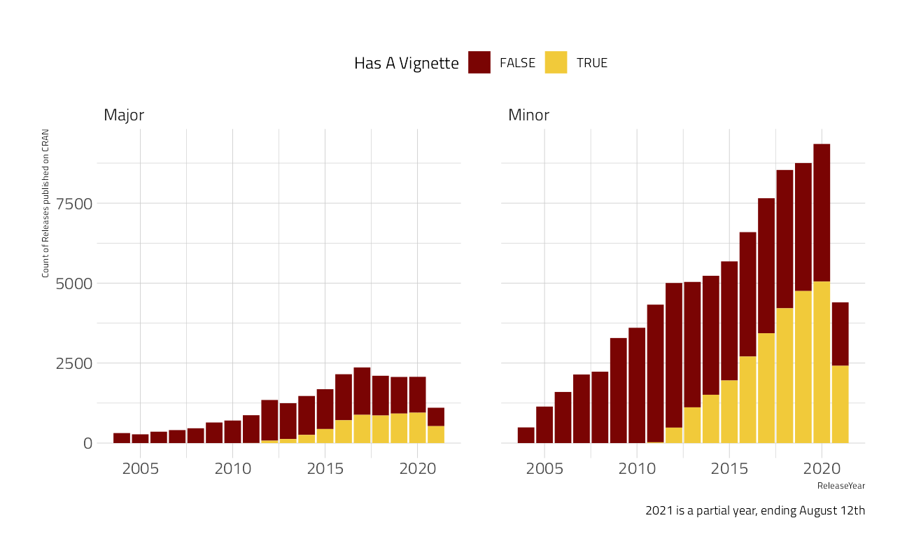

vignette_counts <- cran %>%
  arrange(package, date) %>%
  filter(!is.na(date)) %>%
  group_by(package) %>%
  summarise(
    vignettes = last(VignetteCount),
    born_on = lubridate::year(min(date)),
    age = round(
      lubridate::interval(min(date), Sys.Date()) / lubridate::years(1), 1
    ),
    releases = n(),
    .groups = "drop"
  ) %>%
  inner_join(downloads, by = "package")

vignette_counts %>%
  mutate(package = glue::glue("{ package } \n { vignettes }")) %>%
  ggplot(aes(
    area = count,
    fill = vignettes,
    label = package,
    subgroup = cut_interval(born_on, n = 4)
  )) +
  geom_treemap(show.legend = FALSE) +
  geom_treemap_subgroup_border() +
  geom_treemap_text(aes(color = after_scale(map_chr(fill, best_contrast))),
    place = "top",
    reflow = TRUE
  ) +
  geom_treemap_subgroup_text(
    color = "white",
    alpha = 0.2,
    place = "bottomleft",
    fontface = "italic",
    min.size = 0
  ) +
  labs(
    fill = NULL, title = "Top Most Downloaded R Packages from CRAN",
    subtitle = "Package Name and Number of Vignettes labeled. Size corresponds to the Total Number of Downloads from 14Feb-15Mar2022.",
    caption = "Data Source: Robert Flight and cranlogs"
  ) +
  theme(legend.position = "none")

tweetrmd::include_tweet("https://twitter.com/jim_gruman/status/1504143273925148672")

This week’s #TidyTuesday on the most popular #rstats CRAN extension package vignettes, also using the cranlogs popularity figures.

Code: https://t.co/AY9Y0JfsYe pic.twitter.com/rcJ5OVFXTA

— Jim Gruman📚🚵‍♂️⚙📈 (@jim_gruman) March 16, 2022

Let’s build on Julia Silge’s video from this week on Machine Learning with tidymodels.

A regression model of counts is often best modeled with the poisson distribution

poisson_wf <- workflow(vignettes ~ releases, poisson_reg())

fit(poisson_wf, data = vignette_counts)

== Workflow [trained] ==========================================================
Preprocessor: Formula
Model: poisson_reg()

-- Preprocessor ----------------------------------------------------------------
vignettes ~ releases

-- Model -----------------------------------------------------------------------

Call:  stats::glm(formula = ..y ~ ., family = stats::poisson, data = data)

Coefficients:
(Intercept)     releases  
    0.19996      0.02019  

Degrees of Freedom: 99 Total (i.e. Null);  98 Residual
Null Deviance:      341.8 
Residual Deviance: 285.4    AIC: 452.5

Let’s try a zero inflated model, with the zero inflated terms, that is, those with a probability of being zero, modeled by born_on year.

zip_spec <- poisson_reg() %>% set_engine("zeroinfl")

zip_wf <- workflow() %>%
  add_model(zip_spec, formula = vignettes ~ releases | releases) %>%
  add_variables(
    outcomes = vignettes,
    predictors = c(releases, born_on)
  )

fit(zip_wf, data = vignette_counts)

== Workflow [trained] ==========================================================
Preprocessor: Variables
Model: poisson_reg()

-- Preprocessor ----------------------------------------------------------------
Outcomes: vignettes
Predictors: c(releases, born_on)

-- Model -----------------------------------------------------------------------

Call:
pscl::zeroinfl(formula = vignettes ~ releases | releases, data = data)

Count model coefficients (poisson with log link):
(Intercept)     releases  
     0.9023       0.0120  

Zero-inflation model coefficients (binomial with logit link):
(Intercept)     releases  
    0.47398     -0.04801  

Bootstrapping to better understand the model coefficients for inference

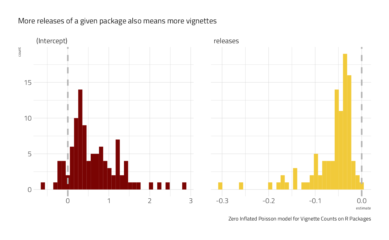
folds <- bootstraps(vignette_counts, times = 100)

Let’s speed this up as best as we can with parallel processing.

all_cores <- parallelly::availableCores(omit = 1)
all_cores

system 
    11 

future::plan("multisession", workers = all_cores) # on Windows

get_coefficients <- function(x) {
  extract_fit_engine(x) %>%
    tidy(type = "zero")
}

ctrl <- control_resamples(
  extract = get_coefficients
)

zip_res <- fit_resamples(zip_wf,
  folds,
  control = ctrl
)

For all of the bootstraps, what is the estimate of the coefficient statistic? Let’s make a plot:

zip_res %>%
  select(id, .extracts) %>%
  unnest(.extracts) %>%
  unnest(.extracts) %>%
  ggplot(aes(x = estimate, fill = term)) +
  geom_histogram(show.legend = FALSE, bins = 35) +
  facet_wrap(~term, scales = "free_x") +
  geom_vline(
    xintercept = 0,
    lty = 2,
    size = 1.2,
    color = "gray70"
  ) +
  labs(
    caption = "Zero Inflated Poisson model for Vignette Counts on R Packages",
    subtitle = "More releases of a given package also means more vignettes"
  )

Session information

sessionInfo()

R version 4.1.2 (2021-11-01)
Platform: x86_64-w64-mingw32/x64 (64-bit)
Running under: Windows 10 x64 (build 22000)

Matrix products: default

locale:
[1] LC_COLLATE=English_United States.1252 
[2] LC_CTYPE=English_United States.1252   
[3] LC_MONETARY=English_United States.1252
[4] LC_NUMERIC=C                          
[5] LC_TIME=English_United States.1252    

attached base packages:
[1] stats     graphics  grDevices utils     datasets  methods   base     

other attached packages:
 [1] pscl_1.5.5           vctrs_0.3.8          rlang_1.0.1         
 [4] poissonreg_0.2.0     yardstick_0.0.9      workflowsets_0.1.0  
 [7] workflows_0.2.4      tune_0.1.6           rsample_0.1.1       
[10] recipes_0.2.0        parsnip_0.2.0        modeldata_0.1.1     
[13] infer_1.0.0          dials_0.1.0          scales_1.1.1        
[16] broom_0.7.12         tidymodels_0.1.4     treemapify_2.5.5    
[19] grumanlib_0.1.0.9999 forcats_0.5.1        stringr_1.4.0       
[22] dplyr_1.0.8          purrr_0.3.4          readr_2.1.2         
[25] tidyr_1.2.0          tibble_3.1.6         ggplot2_3.3.5       
[28] tidyverse_1.3.1      workflowr_1.7.0     

loaded via a namespace (and not attached):
  [1] readxl_1.3.1       backports_1.4.1    systemfonts_1.0.4 
  [4] selectr_0.4-2      plyr_1.8.6         tidytuesdayR_1.0.2
  [7] splines_4.1.2      listenv_0.8.0      usethis_2.1.5     
 [10] digest_0.6.29      foreach_1.5.2      htmltools_0.5.2   
 [13] viridis_0.6.2      fansi_1.0.2        magrittr_2.0.2    
 [16] memoise_2.0.1      tzdb_0.2.0         globals_0.14.0    
 [19] ggfittext_0.9.1    modelr_0.1.8       gower_1.0.0       
 [22] vroom_1.5.7        R.utils_2.11.0     hardhat_0.2.0     
 [25] colorspace_2.0-3   rvest_1.0.2        textshaping_0.3.6 
 [28] haven_2.4.3        xfun_0.29          prismatic_1.1.0   
 [31] callr_3.7.0        crayon_1.5.0       jsonlite_1.8.0    
 [34] survival_3.2-13    iterators_1.0.14   glue_1.6.2        
 [37] gtable_0.3.0       ipred_0.9-12       R.cache_0.15.0    
 [40] tweetrmd_0.0.9     future.apply_1.8.1 DBI_1.1.2         
 [43] Rcpp_1.0.8.2       viridisLite_0.4.0  bit_4.0.4         
 [46] GPfit_1.0-8        lava_1.6.10        prodlim_2019.11.13
 [49] httr_1.4.2         ellipsis_0.3.2     farver_2.1.0      
 [52] pkgconfig_2.0.3    R.methodsS3_1.8.1  nnet_7.3-16       
 [55] sass_0.4.0         dbplyr_2.1.1       utf8_1.2.2        
 [58] here_1.0.1         labeling_0.4.2     tidyselect_1.1.2  
 [61] DiceDesign_1.9     later_1.3.0        munsell_0.5.0     
 [64] cellranger_1.1.0   tools_4.1.2        cachem_1.0.6      
 [67] cli_3.2.0          generics_0.1.2     evaluate_0.15     
 [70] fastmap_1.1.0      yaml_2.3.4         ragg_1.2.2        
 [73] bit64_4.0.5        processx_3.5.2     knitr_1.37        
 [76] fs_1.5.2           future_1.24.0      whisker_0.4       
 [79] R.oo_1.24.0        xml2_1.3.3         compiler_4.1.2    
 [82] rstudioapi_0.13    curl_4.3.2         cranlogs_2.1.1    
 [85] reprex_2.0.1       lhs_1.1.4          bslib_0.3.1       
 [88] stringi_1.7.6      highr_0.9          ps_1.6.0          
 [91] lattice_0.20-45    Matrix_1.3-4       styler_1.7.0      
 [94] conflicted_1.1.0   pillar_1.7.0       lifecycle_1.0.1   
 [97] furrr_0.2.3        jquerylib_0.1.4    httpuv_1.6.5      
[100] R6_2.5.1           promises_1.2.0.1   gridExtra_2.3     
[103] parallelly_1.30.0  codetools_0.2-18   MASS_7.3-54       
[106] assertthat_0.2.1   rprojroot_2.0.2    withr_2.5.0       
[109] parallel_4.1.2     hms_1.1.1          grid_4.1.2        
[112] rpart_4.1-15       timeDate_3043.102  class_7.3-19      
[115] rmarkdown_2.13     git2r_0.29.0       getPass_0.2-2     
[118] pROC_1.18.0        lubridate_1.8.0