Crop Yields
August 31, 2020
Last updated: 2021-09-21
Checks: 7 0
Knit directory: myTidyTuesday/
This reproducible R Markdown analysis was created with workflowr (version 1.6.2). The Checks tab describes the reproducibility checks that were applied when the results were created. The Past versions tab lists the development history.
Great! Since the R Markdown file has been committed to the Git repository, you know the exact version of the code that produced these results.
Great job! The global environment was empty. Objects defined in the global environment can affect the analysis in your R Markdown file in unknown ways. For reproduciblity it’s best to always run the code in an empty environment.
The command set.seed(20210907) was run prior to running the code in the R Markdown file. Setting a seed ensures that any results that rely on randomness, e.g. subsampling or permutations, are reproducible.
Great job! Recording the operating system, R version, and package versions is critical for reproducibility.
Nice! There were no cached chunks for this analysis, so you can be confident that you successfully produced the results during this run.
Great job! Using relative paths to the files within your workflowr project makes it easier to run your code on other machines.
Great! You are using Git for version control. Tracking code development and connecting the code version to the results is critical for reproducibility.
The results in this page were generated with repository version 61abcc4. See the Past versions tab to see a history of the changes made to the R Markdown and HTML files.
Note that you need to be careful to ensure that all relevant files for the analysis have been committed to Git prior to generating the results (you can use wflow_publish or wflow_git_commit). workflowr only checks the R Markdown file, but you know if there are other scripts or data files that it depends on. Below is the status of the Git repository when the results were generated:
Ignored files:
    Ignored:    .Rhistory
    Ignored:    .Rproj.user/
    Ignored:    analysis/figure/
    Ignored:    catboost_info/
    Ignored:    data/2021-09-08/
    Ignored:    data/acs_poverty.rds
    Ignored:    data/fmhpi.rds
    Ignored:    data/grainstocks.rds
    Ignored:    data/hike_data.rds
    Ignored:    data/us_states.rds
    Ignored:    data/us_states_hexgrid.geojson
    Ignored:    data/weatherstats_toronto_daily.csv

Untracked files:
    Untracked:  code/work list batch targets.R
    Untracked:  figure/
Note that any generated files, e.g. HTML, png, CSS, etc., are not included in this status report because it is ok for generated content to have uncommitted changes.
These are the previous versions of the repository in which changes were made to the R Markdown (analysis/CropYields.Rmd) and HTML (docs/CropYields.html) files. If you’ve configured a remote Git repository (see ?wflow_git_remote), click on the hyperlinks in the table below to view the files as they were in that past version.
| File | Version | Author | Date | Message |
|---|---|---|---|---|
| Rmd | 61abcc4 | opus1993 | 2021-09-21 | adopt new viridis color schema |
TidyTuesday
Join the R4DS Online Learning Community in the weekly #TidyTuesday event! Every week we post a raw dataset, a chart or article related to that dataset, and ask you to explore the data. While the dataset will be “tamed”, it will not always be tidy! As such you might need to apply various R for Data Science techniques to wrangle the data into a true tidy format. The goal of TidyTuesday is to apply your R skills, get feedback, explore other’s work, and connect with the greater #RStats community! As such we encourage everyone of all skills to participate!
Load the weekly Data
Dowload the weekly data and make available in the tt object.
tt <- tidytuesdayR::tt_load("2020-09-01")
    Downloading file 1 of 5: `arable_land_pin.csv`
    Downloading file 2 of 5: `cereal_crop_yield_vs_fertilizer_application.csv`
    Downloading file 3 of 5: `cereal_yields_vs_tractor_inputs_in_agriculture.csv`
    Downloading file 4 of 5: `key_crop_yields.csv`
    Downloading file 5 of 5: `land_use_vs_yield_change_in_cereal_production.csv`
Readme
Take a look at the readme for the weekly data to get insight on the dataset. This includes a data dictionary, source, and a link to an article on the data.
ttGlimpse Data
Take an initial look at the format of the data available.
tt %>%
  map(glimpse)
Wrangle
Explore the data and process it into a nice format for plotting! Access each dataset by name by using a dollarsign after the tt object and then the name of the data set.
nutrient <- tt$cereal_crop_yield_vs_fertilizer_application
nutrient_rates <- nutrient %>%
mutate(
Cereal = `Cereal yield (tonnes per hectare)`,
Nitrogen = `Nitrogen fertilizer use (kilograms per hectare)`, Nitrogen = if_else(is.na(Nitrogen), 0, Nitrogen),
Efficiency = Cereal / Nitrogen, .keep = "unused"
) %>%
filter(Efficiency < 10, !is.na(Code)) %>%
tidyr::nest(data = c(Efficiency, Nitrogen, Cereal, Year)) %>%
mutate(fit = map(.x = data, .f = ~ lm(Efficiency ~ Year, data = .))) %>%
mutate(slope = purrr::map_dbl(.x = fit, .f = ~ broom::tidy(.)$estimate[2])) %>%
tidyr::unnest(data) %>%
group_by(Entity) %>%
mutate(avg_yield = mean(Cereal)) %>%
ungroup()
btm <- quantile(nutrient_rates$slope, probs = c(0.2, 0.8))[1]
top <- quantile(nutrient_rates$slope, probs = c(0.2, 0.8))[2]
nutrient_rates <- nutrient_rates %>%
mutate(
bin = case_when(
slope < btm ~ "Decrease",
slope > top ~ "Increase",
TRUE ~ "Flat"
),
Year = as.integer(Year)
)
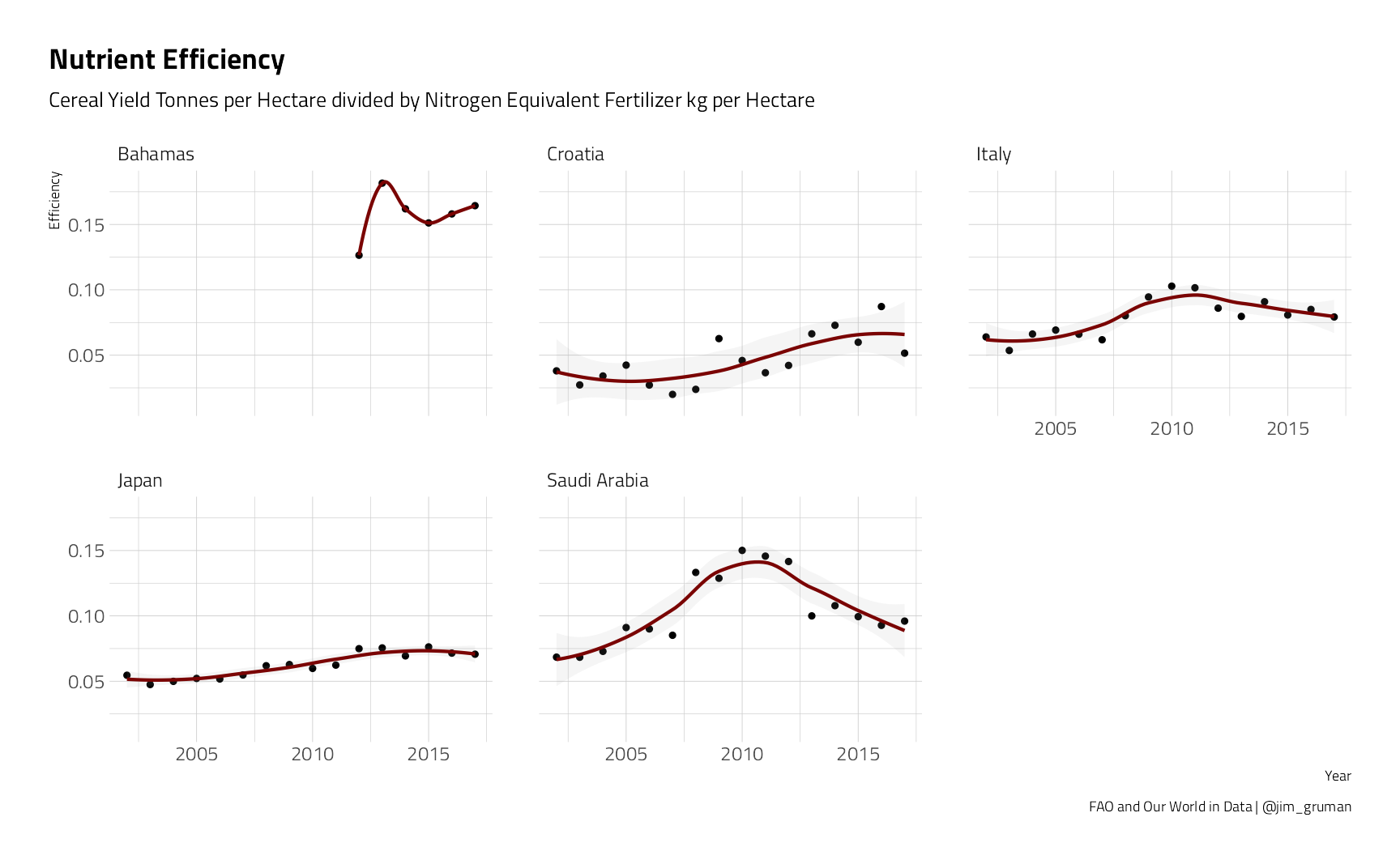
nutrient_rates %>%
filter(bin %in% c("Decrease", "Increase"), avg_yield > 5) %>%
ggplot(aes(Year, Efficiency)) +
geom_point() +
geom_smooth(aes(color = bin),
method = "loess",
formula = "y ~ x",
alpha = 0.1, show.legend = FALSE
) +
scale_x_continuous(n.breaks = 4) +
facet_wrap(~Entity) +
labs(
title = "Nutrient Efficiency",
subtitle = "Cereal Yield Tonnes per Hectare divided by Nitrogen Equivalent Fertilizer kg per Hectare",
caption = "FAO and Our World in Data | @jim_gruman"
)
key_crop_yields <- tt$key_crop_yields

land_use <- tt$land_use_vs_yield_change_in_cereal_production
top_countries <- land_use %>%
janitor::clean_names() %>%
filter(
!is.na(code),
entity != "World"
) %>%
group_by(entity) %>%
filter(year == max(year)) %>%
ungroup() %>%
slice_max(total_population_gapminder, n = 30) %>%
pull(entity)tidy_yields <- key_crop_yields %>%
janitor::clean_names() %>%
pivot_longer(wheat_tonnes_per_hectare:bananas_tonnes_per_hectare,
names_to = "crop",
values_to = "yield"
) %>%
mutate(crop = str_remove(crop, "_tonnes_per_hectare")) %>%
filter(
crop %in% c("wheat", "rice", "maize", "barley"),
entity %in% top_countries,
!is.na(yield)
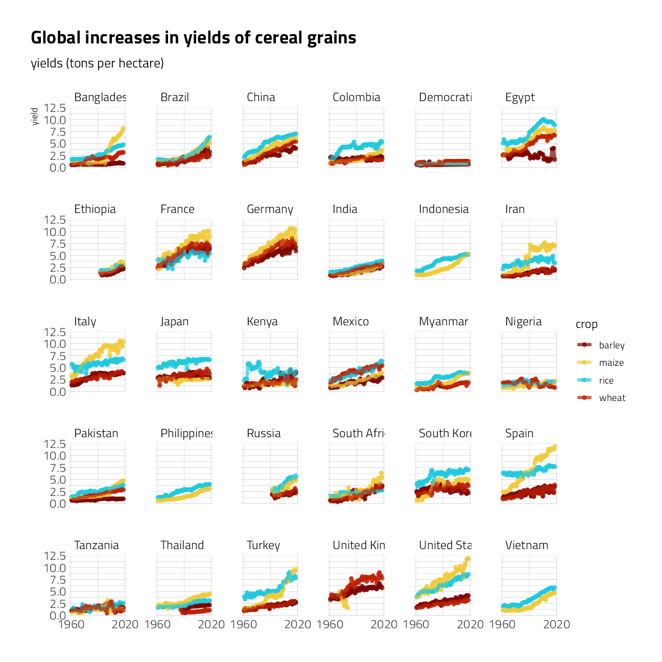
)tidy_yields %>%
ggplot(aes(year, yield, color = crop)) +
geom_point(alpha = 0.7, size = 1.5) +
geom_line(alpha = 0.7, size = 1.5) +
facet_wrap(~entity) +
scale_x_continuous(n.breaks = 2) +
labs(
x = NULL,
subtitle = "yields (tons per hectare)",
title = "Global increases in yields of cereal grains"
)
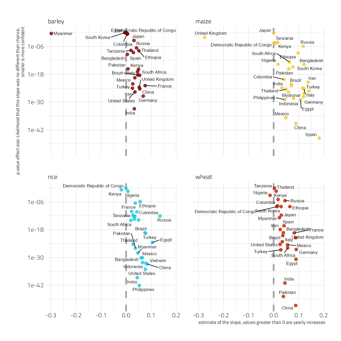
Many Models
Let’s use statistical modeling to measure the country to country differences and changes over time. In this case, a simple linear estimate is useful to compare each country’s growth rates.
This chart depicts the estimate of growth on the x-axis, and the p-value on the y-axis. Consider the p-value the likelihood that the growth estimate is no different than random chance. A smaller p-value is a greater confidence in the effect.
tidy_lm <- tidy_yields %>%
  nest(yields = c(year, yield)) %>%
  mutate(model = map(yields, ~ lm(yield ~ year, data = .x)))

slopes <- tidy_lm %>%
  mutate(coefs = map(model, broom::tidy)) %>%
  unnest(coefs) %>%
  filter(term == "year") %>%
  mutate(p.value = p.adjust(p.value))
slopes %>%
ggplot(aes(estimate, p.value, label = entity)) +
geom_vline(xintercept = 0, lty = 2, size = 1.5, alpha = 0.7, color = "gray50") +
geom_point(aes(color = crop), alpha = 0.8, size = 2.5, show.legend = FALSE) +
ggrepel::geom_text_repel(size = 3) +
scale_y_log10() +
facet_wrap(~crop) +
labs(
y = "p.value effect size: Likelihood that this slope was no different than chance, \nsmaller is more confident",
x = "estimate of the slope, values greater than 0 are yearly increases"
)
sessionInfo()R version 4.1.1 (2021-08-10)
Platform: x86_64-w64-mingw32/x64 (64-bit)
Running under: Windows 10 x64 (build 19043)
Matrix products: default
locale:
[1] LC_COLLATE=English_United States.1252
[2] LC_CTYPE=English_United States.1252
[3] LC_MONETARY=English_United States.1252
[4] LC_NUMERIC=C
[5] LC_TIME=English_United States.1252
attached base packages:
[1] stats graphics grDevices utils datasets methods base
other attached packages:
[1] forcats_0.5.1 stringr_1.4.0 dplyr_1.0.7 purrr_0.3.4
[5] readr_2.0.1 tidyr_1.1.3 tibble_3.1.4 ggplot2_3.3.5
[9] tidyverse_1.3.1 workflowr_1.6.2
loaded via a namespace (and not attached):
[1] readxl_1.3.1 backports_1.2.1 systemfonts_1.0.2
[4] workflows_0.2.3 plyr_1.8.6 selectr_0.4-2
[7] tidytuesdayR_1.0.1 splines_4.1.1 listenv_0.8.0
[10] usethis_2.0.1 digest_0.6.27 foreach_1.5.1
[13] htmltools_0.5.2 yardstick_0.0.8 viridis_0.6.1
[16] parsnip_0.1.7.900 fansi_0.5.0 magrittr_2.0.1
[19] tune_0.1.6 tzdb_0.1.2 recipes_0.1.16
[22] globals_0.14.0 modelr_0.1.8 gower_0.2.2
[25] extrafont_0.17 R.utils_2.10.1 vroom_1.5.5
[28] extrafontdb_1.0 hardhat_0.1.6 rsample_0.1.0
[31] dials_0.0.10 colorspace_2.0-2 ggrepel_0.9.1
[34] rvest_1.0.1 textshaping_0.3.5 haven_2.4.3
[37] xfun_0.26 crayon_1.4.1 jsonlite_1.7.2
[40] survival_3.2-11 iterators_1.0.13 glue_1.4.2
[43] gtable_0.3.0 ipred_0.9-12 R.cache_0.15.0
[46] Rttf2pt1_1.3.9 future.apply_1.8.1 scales_1.1.1
[49] infer_1.0.0 DBI_1.1.1 Rcpp_1.0.7
[52] viridisLite_0.4.0 bit_4.0.4 GPfit_1.0-8
[55] lava_1.6.10 prodlim_2019.11.13 httr_1.4.2
[58] ellipsis_0.3.2 farver_2.1.0 pkgconfig_2.0.3
[61] R.methodsS3_1.8.1 nnet_7.3-16 sass_0.4.0
[64] dbplyr_2.1.1 janitor_2.1.0 utf8_1.2.2
[67] here_1.0.1 labeling_0.4.2 tidyselect_1.1.1
[70] rlang_0.4.11 DiceDesign_1.9 later_1.3.0
[73] munsell_0.5.0 cellranger_1.1.0 tools_4.1.1
[76] cachem_1.0.6 cli_3.0.1 generics_0.1.0
[79] broom_0.7.9 evaluate_0.14 fastmap_1.1.0
[82] yaml_2.2.1 ragg_1.1.3 bit64_4.0.5
[85] knitr_1.34 fs_1.5.0 nlme_3.1-152
[88] future_1.22.1 whisker_0.4 R.oo_1.24.0
[91] xml2_1.3.2 compiler_4.1.1 rstudioapi_0.13
[94] curl_4.3.2 reprex_2.0.1 lhs_1.1.3
[97] bslib_0.3.0 stringi_1.7.4 highr_0.9
[100] gdtools_0.2.3 hrbrthemes_0.8.0 lattice_0.20-44
[103] Matrix_1.3-4 styler_1.6.1 conflicted_1.0.4
[106] vctrs_0.3.8 tidymodels_0.1.3 pillar_1.6.2
[109] lifecycle_1.0.0 furrr_0.2.3 jquerylib_0.1.4
[112] httpuv_1.6.3 R6_2.5.1 promises_1.2.0.1
[115] gridExtra_2.3 parallelly_1.28.1 codetools_0.2-18
[118] MASS_7.3-54 assertthat_0.2.1 rprojroot_2.0.2
[121] withr_2.4.2 mgcv_1.8-36 parallel_4.1.1
[124] hms_1.1.0 grid_4.1.1 rpart_4.1-15
[127] timeDate_3043.102 class_7.3-19 snakecase_0.11.0
[130] rmarkdown_2.11 git2r_0.28.0 pROC_1.18.0
[133] lubridate_1.7.10