Kaggle Feedback Prize - English Language Learning

workflowr

• Summary
• Checks
• Past versions

Last updated: 2022-12-16

Checks: 7 0

Knit directory: myTidyTuesday/

This reproducible R Markdown analysis was created with workflowr (version 1.7.0). The Checks tab describes the reproducibility checks that were applied when the results were created. The Past versions tab lists the development history.

---

R Markdown file: up-to-date

Great! Since the R Markdown file has been committed to the Git repository, you know the exact version of the code that produced these results.

Environment: empty

Great job! The global environment was empty. Objects defined in the global environment can affect the analysis in your R Markdown file in unknown ways. For reproduciblity it’s best to always run the code in an empty environment.

Seed: set.seed(20210907)

The command set.seed(20210907) was run prior to running the code in the R Markdown file. Setting a seed ensures that any results that rely on randomness, e.g. subsampling or permutations, are reproducible.

Session information: recorded

Great job! Recording the operating system, R version, and package versions is critical for reproducibility.

Cache: none

Nice! There were no cached chunks for this analysis, so you can be confident that you successfully produced the results during this run.

File paths: relative

Great job! Using relative paths to the files within your workflowr project makes it easier to run your code on other machines.

Repository version: f0ab5e8

Great! You are using Git for version control. Tracking code development and connecting the code version to the results is critical for reproducibility.

The results in this page were generated with repository version f0ab5e8. See the Past versions tab to see a history of the changes made to the R Markdown and HTML files.

Note that you need to be careful to ensure that all relevant files for the analysis have been committed to Git prior to generating the results (you can use wflow_publish or wflow_git_commit). workflowr only checks the R Markdown file, but you know if there are other scripts or data files that it depends on. Below is the status of the Git repository when the results were generated:

Ignored files:
    Ignored:    .Rhistory
    Ignored:    .Rproj.user/
    Ignored:    data/.Rhistory
    Ignored:    data/2022_11_01.png
    Ignored:    data/2022_11_18.png
    Ignored:    data/CNHI_Excel_Chart.xlsx
    Ignored:    data/Chicago.rds
    Ignored:    data/CommunityTreemap.jpeg
    Ignored:    data/Community_Roles.jpeg
    Ignored:    data/ELL.zip
    Ignored:    data/FM_service_contour_current.zip
    Ignored:    data/SeriesReport-20220414171148_6c3b18.xlsx
    Ignored:    data/Weekly_Chicago_IL_Regular_Reformulated_Retail_Gasoline_Prices.csv
    Ignored:    data/YammerDigitalDataScienceMembership.xlsx
    Ignored:    data/YammerMemberPage.rds
    Ignored:    data/YammerMembers.rds
    Ignored:    data/application_id.feather
    Ignored:    data/df.rds
    Ignored:    data/fit_cohesion.rds
    Ignored:    data/fit_grammar.rds
    Ignored:    data/fit_phraseology.rds
    Ignored:    data/fit_syntax.rds
    Ignored:    data/fit_vocabulary.rds
    Ignored:    data/grainstocks.rds
    Ignored:    data/hike_data.rds
    Ignored:    data/lm_res.rds
    Ignored:    data/raw_contour.feather
    Ignored:    data/raw_weather.RData
    Ignored:    data/sample_submission.csv
    Ignored:    data/submission.csv
    Ignored:    data/test.csv
    Ignored:    data/train.csv
    Ignored:    data/us_states.rds
    Ignored:    data/us_states_hexgrid.geojson
    Ignored:    data/weatherstats_toronto_daily.csv

Untracked files:
    Untracked:  analysis/2022_09_01_kaggle_tabular_playground.qmd
    Untracked:  code/YammerReach.R
    Untracked:  code/autokeras.R
    Untracked:  code/chicago.R
    Untracked:  code/glmnet_test.R
    Untracked:  code/googleCompute.R
    Untracked:  code/work list batch targets.R
    Untracked:  environment.yml
    Untracked:  report.html

Unstaged changes:
    Modified:   analysis/2021_01_19_tidy_tuesday.Rmd
    Modified:   analysis/2021_03_24_tidy_tuesday.Rmd
    Deleted:    analysis/2021_04_20.Rmd
    Deleted:    analysis/2022_02_11_tabular_playground.Rmd
    Deleted:    analysis/2022_04_18.qmd
    Modified:   analysis/Survival.Rmd
    Modified:   analysis/_site.yml
    Modified:   code/_common.R

Note that any generated files, e.g. HTML, png, CSS, etc., are not included in this status report because it is ok for generated content to have uncommitted changes.

---

These are the previous versions of the repository in which changes were made to the R Markdown (analysis/EnglishLanguageLearning.Rmd) and HTML (docs/EnglishLanguageLearning.html) files. If you’ve configured a remote Git repository (see ?wflow_git_remote), click on the hyperlinks in the table below to view the files as they were in that past version.

File	Version	Author	Date	Message
html	f0ab5e8	opus1993	2022-11-29	Build site.
Rmd	c07b02a	opus1993	2022-11-29	wflow_publish("analysis/EnglishLanguageLearning.Rmd")
Rmd	42d2421	opus1993	2022-11-29	add likert and resamples on all metrics
html	b5a9c2b	opus1993	2022-10-15	Build site.
html	fad0136	opus1993	2022-10-15	Build site.
Rmd	73c07de	opus1993	2022-10-15	Kaggle English Language Learning
html	66b10e0	opus1993	2022-10-15	Build site.
Rmd	bb8b757	opus1993	2022-10-15	initial commit of Kaggle English Language Learning

---

The Kaggle Challenge presented here works with a dataset that comprises argumentative essays (the ELLIPSE corpus) written by 8th-12th grade English Language Learners (ELLs). The essays have been scored on six measures: cohesion, syntax, vocabulary, phraseology, grammar, and conventions.

Each measure represents a component of writing proficiency, ranging from 1.0 to 5.0 in increments of 0.5. Our task is to predict the score of each measure by essay.

This is the rubric that was used to grade the essays. Two people did the work independently, and then the scores were compared for alignment.

Preprocessing

Natural Language Processing techniques offer a wide variety of tools to approach this problem. The Kaggle host is requiring that the model run as a standalone, without internet assistance. They also ask for a parsimonous, explainable model.

We will start with exploring the predictive potential of the text count features, like numbers of words, distinct words, and spaces.

Unsupervised topic grouping categories may be useful for measures like conventions or grammar. In this case, we will start with Latent Dirichlet allocation (LDA).

Individual words may have predictive power, but they could be so sparse as to be difficult to separate from the background noise. Consider words like ain’t and phrases taken from other languages.

Bringing in a sentiment dictionary may add predictive power to some measures, along with helping to count miss-spellings. Word embeddings like Glove or Huggingface could also better characterize meaning.

Modeling

Many developers are tempted to jump into (CNN / LSTM) deep learning, but the number of essays is really pretty small for a deep learning run on their own. Another approach could leverage the pre-trained embeddings in one of the BERTs. The current Kaggle leaderboard is full of them. Even so, the standings will shift in a huge way after the full test set calculations appear because of overfitting and imbalance.

The GloVe pre-trained word vectors provide word embeddings created on existing document corpus, and are provided as a pre-processor using varying numbers of tokens. See Jeffrey Pennington, Richard Socher, and Christopher D. Manning. 2014. GloVe: Global Vectors for Word Representation. for details.

I spent a few evenings with the torch/brulee approach on tidymodels, but discovered that modeling time consumed would be significant and the results were not better than random forests on engineered features with case weights based on inverse proportions of the metric values.

I ultimately settled on the xgboost approach here. No doubt it can still overfit on specific words and text attributes, like the number of unique words.

One last point. I believe that the Essay Scoring is done by humans in a way where the metrics are judged together, and not entirely independently. In other words, low grammar and low cohesion are related.

suppressPackageStartupMessages({
library(tidyverse)
  
library(tidymodels)
library(text2vec) # for topic modeling

library(tidytext)
library(textrecipes)

})

tidymodels::tidymodels_prefer()

theme_set(theme_minimal())

Let’s read the data from Kaggle’s csv’s into dataframes.

train_essays_raw <- read_csv(here::here("data","train.csv"),
                         show_col_types = FALSE) 

submit_essays_raw <- read_csv(here::here("data","test.csv"),
                          show_col_types = FALSE) 

outcomes = names(train_essays_raw)[3:8]

dim(train_essays_raw)

[1] 3911    8

The essay metrics score distributions resemble ordinal Likert scales. One way to illustrate the counts at each level is this bar chart:

stage1 <- train_essays_raw |>
  select(cohesion:conventions) |>
  pivot_longer(cols = everything(),
               names_to = "metric",
               values_to = "ans") |>
  group_by(ans, metric) |>
  summarize(n = n(),
            .groups = "drop") |>
  group_by(metric) |>
  mutate(per = n / sum(n)) |>
  mutate(
    text = paste0(formatC(
      100 * per, format = "f", digits = 0
    ), "%"),
    cs = cumsum(per),
    offset = sum(per[1:(floor(n() / 2))]) + (n() %% 2) * 0.5 * (per[ceiling(n() /
                                                                              2)]),
    xmax = -offset + cs,
    xmin = xmax - per
  ) |>
  ungroup()

gap <- 0.2

stage2 <- stage1 %>%
  left_join(
    stage1 %>%
      group_by(metric) %>%
      summarize(max.xmax = max(xmax)) %>%
      mutate(r = row_number(max.xmax)),
    by = "metric"
  ) %>%
  arrange(desc(r)) %>%
  mutate(ymin = r - (1 - gap) / 2,
         ymax = r + (1 - gap) / 2)

ggplot(stage2) +
  geom_vline(xintercept = 0) +
  geom_rect(aes(
    xmin = xmin,
    xmax = xmax,
    ymin = ymin,
    ymax = ymax,
    fill = factor(ans)
  )) +
  geom_text(aes(
    x = (xmin + xmax) / 2,
    y = (ymin + ymax) / 2,
    label = text
  ),
  size = 3,
  check_overlap = TRUE) +
  scale_x_continuous(
    "",
    labels = percent,
    breaks = seq(-0.6, 0.65, len = 6),
    limits = c(-0.6, 0.65)
  ) +   scale_y_continuous(
    "",
    breaks = 1:n_distinct(stage2$metric),
    labels = rev(stage2 %>% distinct(metric) %>% .$metric)
  ) +
  scale_fill_brewer("Score", palette = "BrBG") +
  labs(title = "Training set Essay Ratings")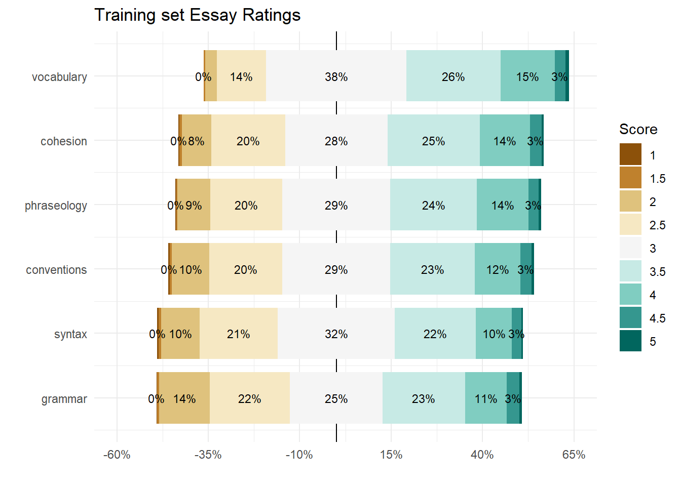

Essays with more words, or more sentences, do not necessarily score better.

te_long <- train_essays_raw |>
  pivot_longer(cols = cohesion:conventions,
               names_to = "metric",
               values_to = "value") |>
  mutate(metric = as.factor(metric),
         value = as.factor(value))

te_long |> 
  group_by(n_words = ggplot2::cut_interval(
    tokenizers::count_words(full_text), 
    length = 200),
    metric, value) |> 
  summarise(`Number of essays` = n(),
            .groups = "drop") |> 
  ggplot(aes(n_words, `Number of essays`, fill = as.factor(value))) +
  geom_col() +
  scale_x_discrete(guide = guide_axis(n.dodge = 2)) +
  facet_wrap(vars(metric)) +
  scale_fill_brewer("Score", palette = "BrBG") +
  labs(x = "Number of words per essay",
       y = "Number of essays",
       fill = "Score")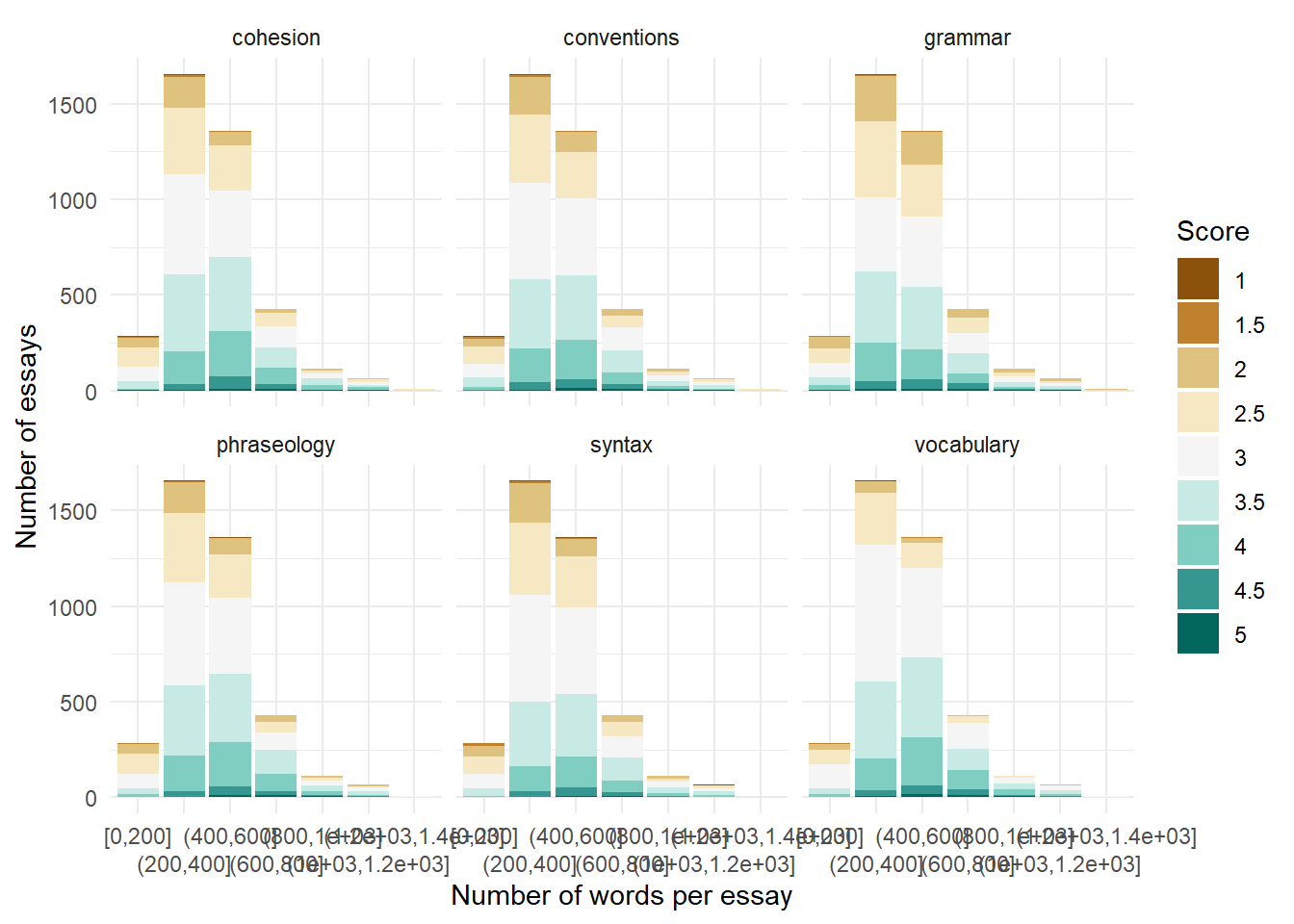

te_long |> 
  group_by(n_words = ggplot2::cut_interval(
    tokenizers::count_sentences(full_text), length = 20),
    metric, value) |> 
  summarise(`Number of essays` = n(),
            .groups = "drop") |> 
  ggplot(aes(n_words, `Number of essays`, fill = as.factor(value))) +
  geom_col() +
  scale_x_discrete(guide = guide_axis(n.dodge = 2)) +
  facet_wrap(vars(metric)) +
  scale_fill_brewer("Score", palette = "BrBG") +
  labs(x = "Number of sentences per essay",
       y = "Number of essays",
       fill = "Score")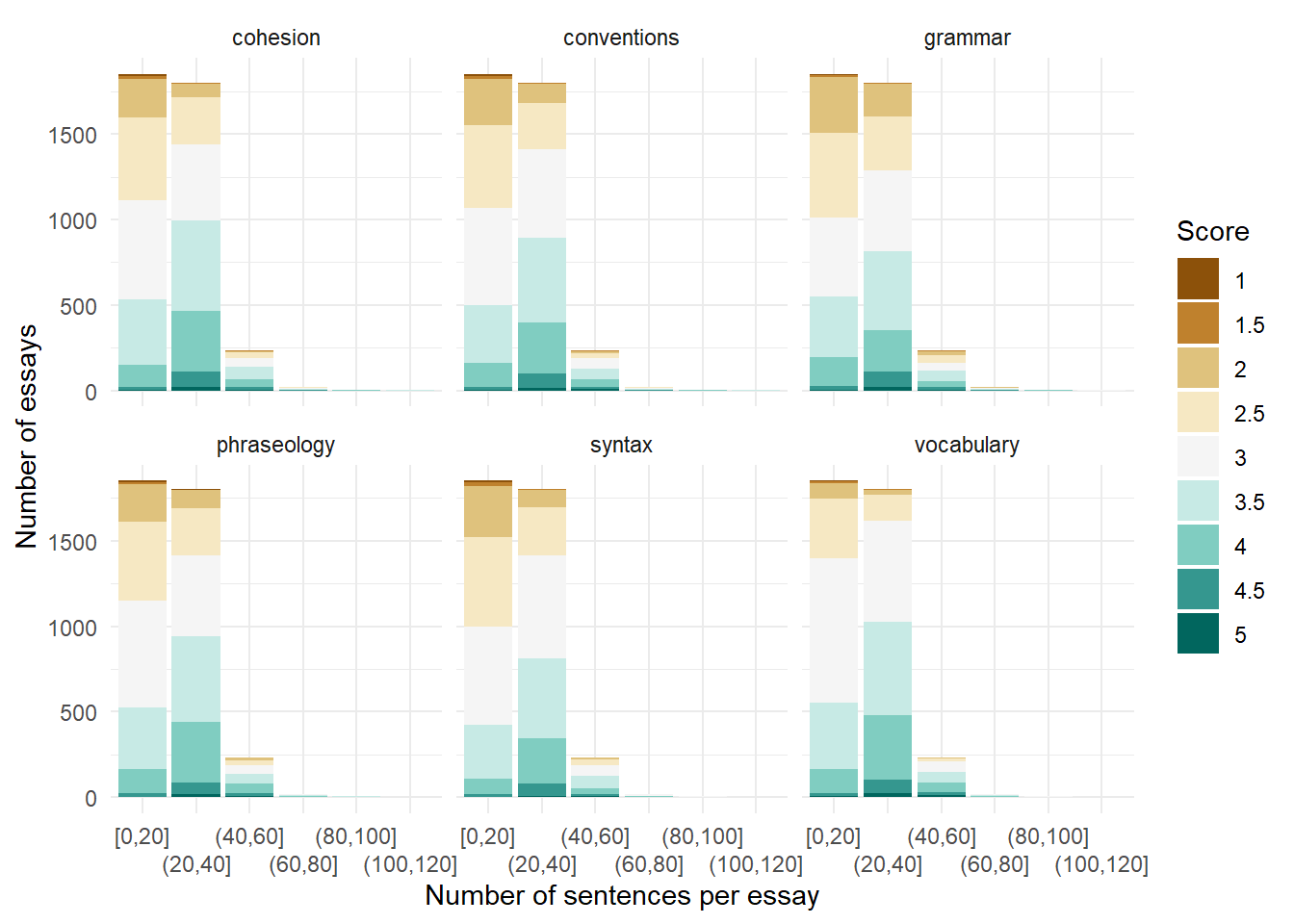

What words from the dialogue have the highest log odds of coming from each level of each outcome? Do the individual words have predictive power?

plot_log_odds <- function(outcome = "cohesion"){

train_essays_raw |>
  tidytext::unnest_tokens(word, full_text) |> 
  count(level = factor(.data[[outcome]]), word, sort = TRUE) |>   
  tidylo::bind_log_odds(level, word, n) |> 
  filter(n > 20) |> 
  group_by(level) |> 
  slice_max(log_odds_weighted, n = 10) |> 
  mutate(word = reorder_within(word, log_odds_weighted, level)) %>%
  ggplot(aes(log_odds_weighted, word, fill = level)) +
  geom_col(show.legend = FALSE) +
  facet_wrap(vars(level), scales = "free") +
  scale_fill_brewer("Score", palette = "BrBG") +
  scale_y_reordered() +
  labs(y = NULL, title = glue::glue("{outcome} log odds words"))  
    
}

map(outcomes, plot_log_odds)

[[1]]

[[2]]

[[3]]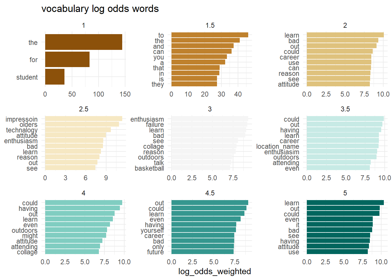

[[4]]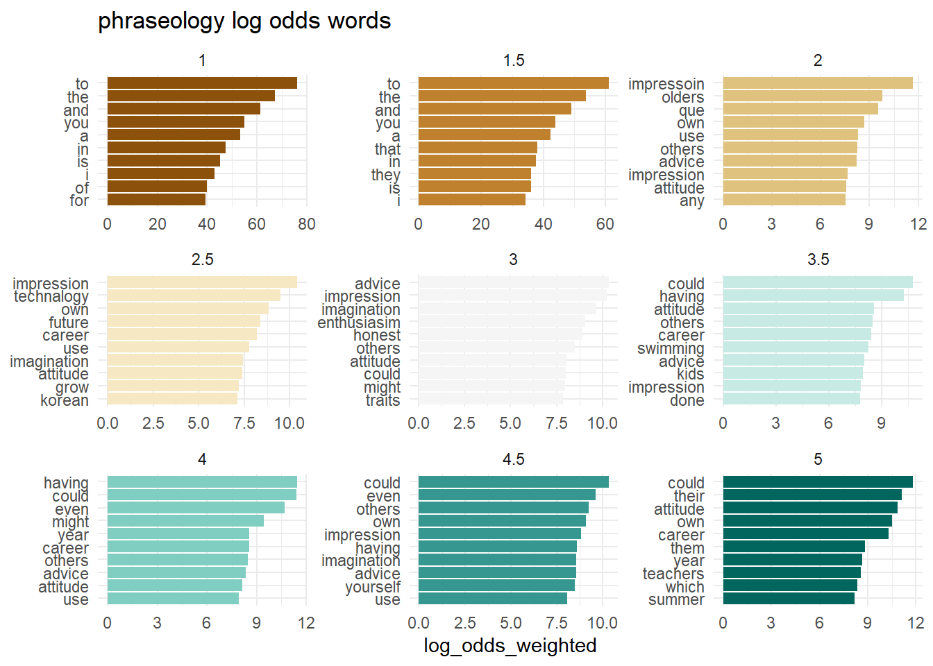

[[5]]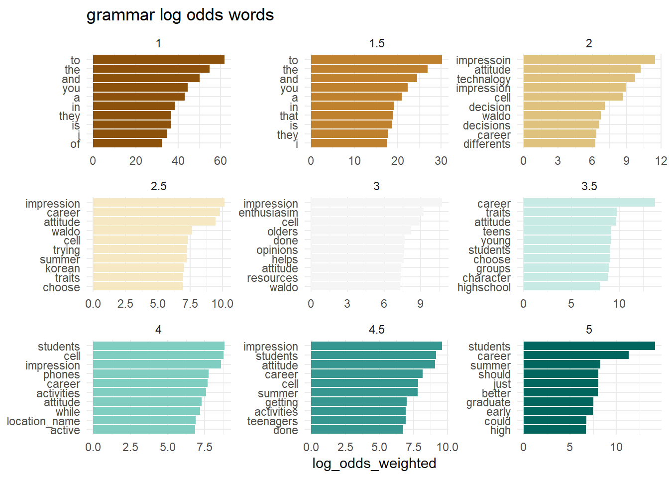

[[6]]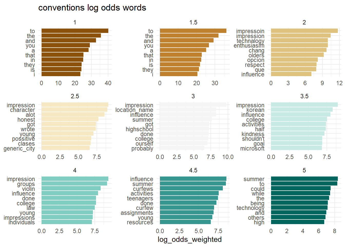

To some extent, the answer may be yes.

Let’s also take a look at outcome pairwise correlations.

train_essays_raw |> 
  corrr::correlate(
    quiet = TRUE
  ) %>%
  corrr::rearrange() %>%
  corrr::shave() %>%
  corrr::rplot(print_cor = TRUE,
               colors = brewer_pal(palette = "BrBG")(5)) +
  scale_x_discrete(guide = guide_axis(n.dodge = 3))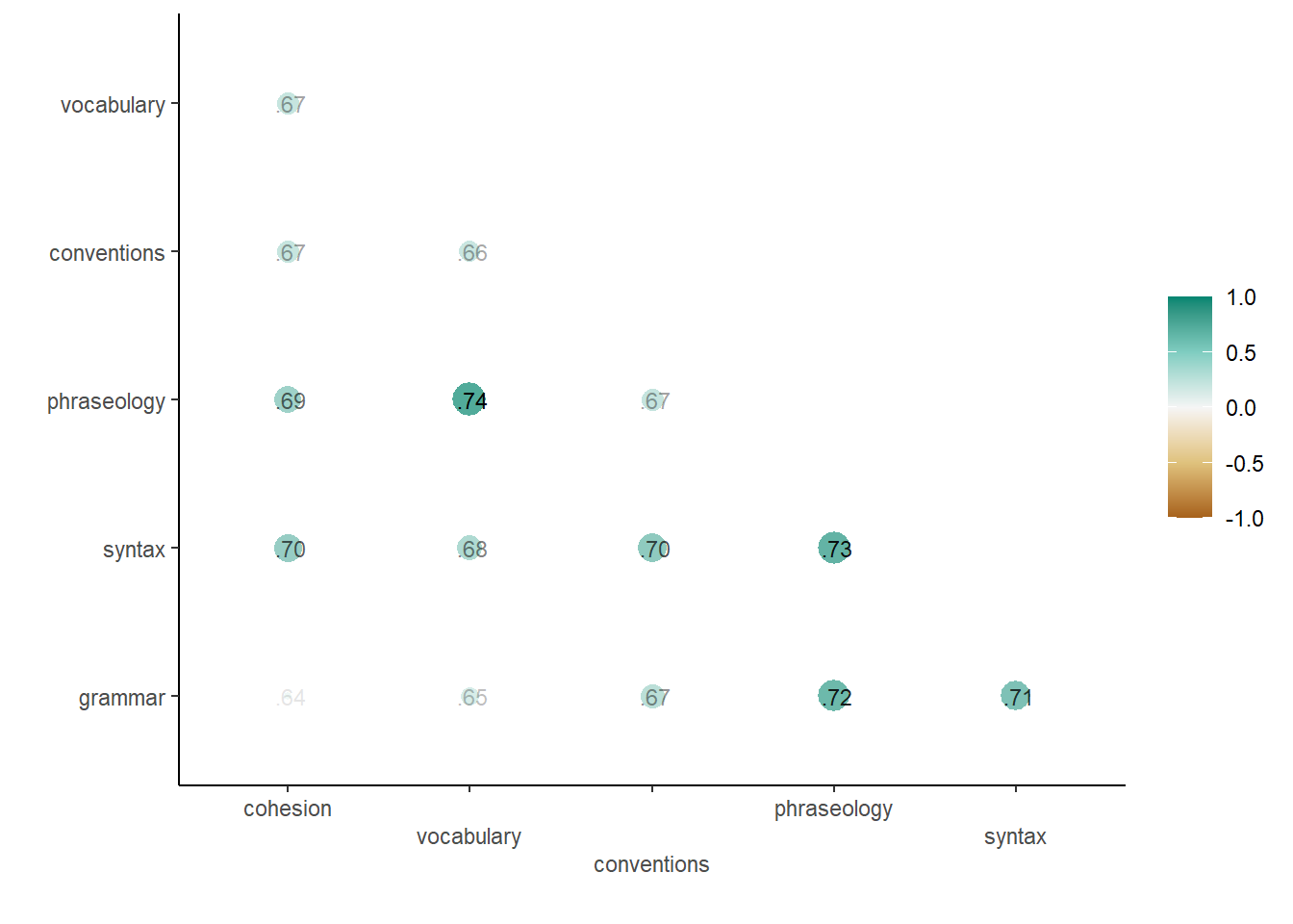

• Vocabulary and Phraseology (0.74) track together.
• Phraseology and Syntax (0.73) track together.
• Praseology and Grammar (0.72) track together.

Avoiding overfitting to the training data is critical to achieving a strong score. We are going to use resampling to have some indication that our model generalizes to new essays. Care must be exercised to be sure that members of the hold out folds are not also found in the training folds.

Latent Dirichlet allocation (LDA) is an unsupervised generative statistical model that explains a set of observations through unobserved groups, and the content of each group may explain why some parts of the data are similar.

I’d like to explore the use of inverse probability weights because there are so few essays with scores at the highest and lowest levels. When survey respondents have different probabilities of selection, (inverse) probability weights help reduce bias in the results.

I am making us of metaprogramming techniques to pass text vector column names into the formula and case weights functions to re-use them for each metric.

tokens = text2vec::word_tokenizer(tolower(train_essays_raw$full_text))

it = text2vec::itoken(tokens, ids = train_essays_raw$text_id, progressbar = FALSE)

v = text2vec::create_vocabulary(it)

dtm = text2vec::create_dtm(it, text2vec::vocab_vectorizer(v), type = "RsparseMatrix")

lda_model <- text2vec::LDA$new(n_topics = 30)

case_weight_builder <- function(data, outcome) {
  data %>%
    inner_join(data %>%
                 count(.data[[outcome]],
                       name = "case_wts"),
               by = glue::glue("{ outcome }")) %>%
    mutate(case_wts = importance_weights(max(case_wts) / case_wts))
}

recipe_builder <- function(outcome = "cohesion") {
  rec <- recipe(
    formula(glue::glue("{ outcome } ~ .")),
    data = train_essays_raw |>
      select({
        {
          outcome
        }
      }, full_text) |>
      case_weight_builder(outcome)
  ) |>
    step_textfeature(full_text,
                     keep_original_cols = TRUE) |>
    step_rename_at(starts_with("textfeature_"),
                   fn = ~ gsub("textfeature_full_text_", "", .)) %>%
    step_tokenize(full_text) %>%
    step_lda(full_text,
             lda_models = lda_model,
             keep_original_cols = TRUE) %>%
    step_word_embeddings(
      full_text,
      aggregation = "sum",
      embeddings = textdata::embedding_glove27b(dimensions = 200)
    ) |>
    step_zv(all_numeric_predictors()) |>
    step_normalize(all_numeric_predictors())
  
  return(rec)
  
}


multiclass_recipe_builder <- function(outcome = "cohesion") {
  rec <- recipe(formula(glue::glue("{ outcome } ~ .")),
                data = classification_train_df) |>
    step_textfeature(full_text,
                     keep_original_cols = TRUE) |>
    step_rename_at(starts_with("textfeature_"),
                   fn = ~ gsub("textfeature_full_text_", "", .)) %>%
    step_tokenize(full_text) %>%
    step_lda(full_text,
             lda_models = lda_model,
             keep_original_cols = TRUE) %>%
    step_word_embeddings(
      full_text,
      aggregation = "sum",
      embeddings = textdata::embedding_glove27b(dimensions = 200)
    ) |>
    step_zv(all_numeric_predictors()) |>
    step_normalize(all_numeric_predictors())
  
  return(rec)
  
}

plot_preds <- function(dat, outcome){

dat |> 
  ggplot(aes(x = {{outcome}}, y = .pred)) +
  geom_point(alpha = 0.15) +
  geom_abline(color = "red") +
  coord_obs_pred() 

}

As mentioned above, the model specification is xgboost for regression to predict a continuous outcome that resembles ordinal classes.

xgb_spec <-
  boost_tree(
    mtry = 50,  # 75L
    trees = 1000L,
    tree_depth = 9, # 6L
    learn_rate = 0.01,  # originally 0.1
    min_n = 39L,  # 20L
    loss_reduction = 0
  ) |> 
  set_engine('xgboost') |> 
  set_mode('regression')

svm_spec <- svm_linear() |> 
  set_engine("LiblineaR") |> 
  set_mode("classification")  

To speed the computations let’s enable a parallel backend.

all_cores <- parallelly::availableCores(omit = 1)
all_cores

system 
    11 

#  
future::plan("multisession", workers = all_cores) # on Windows

Modeling

Cohesion

We fit for cohesion first using an xgboost regression, using case weights to adjust for the frequency of occurrence of each value of cohesion.

outcome <- outcomes[1]

regression_train_df <- train_essays_raw  |> 
                select(!!outcome, full_text) |> 
                case_weight_builder(outcome)

regression_wf <- workflow(recipe_builder(outcome = outcome), xgb_spec) |> 
       add_case_weights(case_wts)

folds <- vfold_cv(regression_train_df, strata = {{outcome}})

set.seed(42)  
rs <- fit_resamples(
  regression_wf,
  folds,
  control = control_resamples(save_pred = TRUE))

as(<dgTMatrix>, "dgCMatrix") is deprecated since Matrix 1.5-0; do as(., "CsparseMatrix") instead

collect_metrics(rs) |> arrange(mean)

collect_predictions(rs) |> 
  plot_preds(.data[[outcome]]) +
  labs(y = "Predicted",
       title = paste0(outcome, " predictions against essays in held out folds"),
       subtitle = "The highest and lowest essays are not predicted well")

train_essays_raw[

collect_predictions(rs) |> 
  mutate(residual = .data[[outcome]] - .pred) |> 
  arrange(desc(abs(residual))) |> 
  slice_head(n = 5) |> 
  pull(.row)

, ] |> 
  select(full_text)

regression_fit <- parsnip::fit(regression_wf, 
                     regression_train_df)

Identifying examples with especially poor performance can help us follow up and investigate why these specific predictions are poor. Conceptually, its easy for a baseline know-nothing model to assign all essays to the median score of 3. The predictive power is in the ability to model the essays that are not 3 into buckets higher and lower than 3.

Because the ratings are a form of ordinal value, or even a likert scale, we will ensemble a second classification model that includes the output of the regression.

classification_train_df <- train_essays_raw  |> 
                select({{outcome}}, full_text) |> 
                bind_cols(
                  predict(
                    regression_fit,
                    regression_train_df
                  )
                ) |> 
               rename(regression_pred = .pred) |> 
               mutate({{outcome}} := factor(.data[[outcome]]))

classification_wf <- workflow(multiclass_recipe_builder(outcome = outcome), svm_spec) 

folds <- vfold_cv(classification_train_df, strata = !!outcome)

set.seed(42)  
rs <- fit_resamples(
  classification_wf,
  folds,
  metrics = metric_set(kap, accuracy),
  control = control_resamples(save_pred = TRUE))

collect_metrics(rs) |> arrange(mean)

collect_predictions(rs) |> 
  ggplot(aes(x = .data[[outcome]], y = abs(as.numeric(.data[[outcome]]) - as.numeric(.pred_class))/2)) +
  geom_violin() +
  scale_y_continuous(breaks = seq(-5,5,0.5)) +
  labs(y = "Residuals",
       title = "{{outcome}} Residual errors for essays in held out folds",
       subtitle = "The highest and lowest essays are still not predicted well")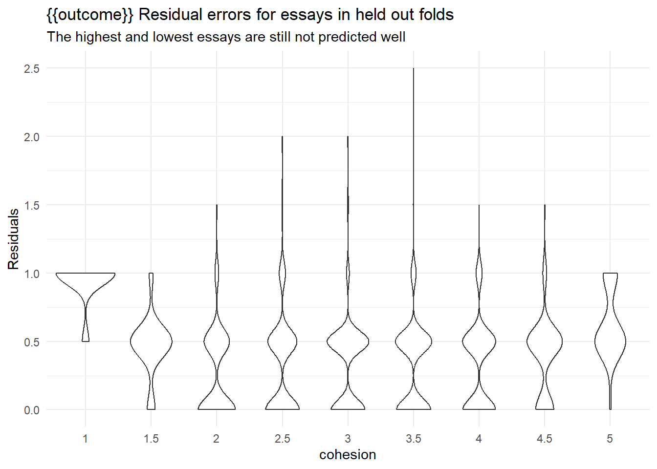

train_essays_raw[

collect_predictions(rs) |> 
  mutate(residual = as.numeric(.data[[outcome]]) - as.numeric(.pred_class)) |> 
  arrange(desc(abs(residual))) |> 
  slice_head(n = 5) |> 
  pull(.row)

, ] |> 
  select(full_text, {{outcome}})

collect_predictions(rs) |> 
  rmse(truth = as.numeric(.data[[outcome]])/2, estimate = as.numeric(.pred_class)/2)

Results here aren’t great, but they are more are less competitive with the leaderboard figures.

The final fitting ensembles both the regression and classification fits, and makes a prediction on the submission essays.

classification_fit <- parsnip::fit(classification_wf,
                                   classification_train_df)

extract_fit_engine(regression_fit) |> 
  vip::vip(num_features = 20)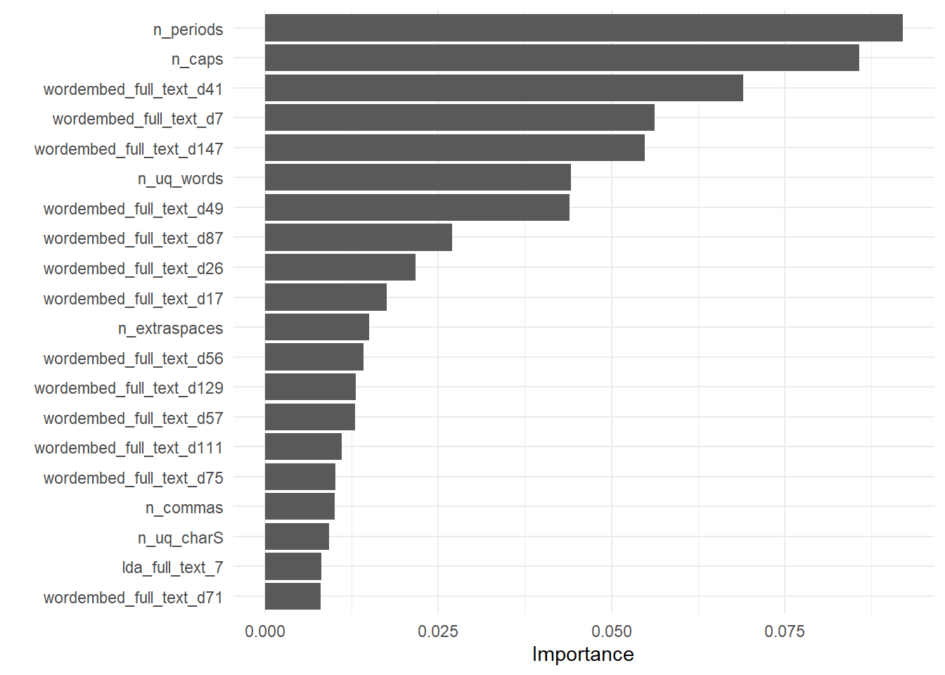

submission <- predict(
  classification_fit,
  
  submit_essays_raw |>
    bind_cols(predict(regression_fit, submit_essays_raw)) |>
    rename(regression_pred = .pred)
) |>
  transmute({{outcome}} := .pred_class)

Warning in get_dtm(corp): dtm has 0 rows. Empty iterator?

Warning in get_dtm(corp): dtm has 0 rows. Empty iterator?

submission

Syntax

We fit for syntax first using an xgboost regression, using case weights to adjust for the frequency of occurrence of each value of syntax.

outcome <- outcomes[2]

regression_train_df <- train_essays_raw  |> 
                select(!!outcome, full_text) |> 
                case_weight_builder(outcome)

regression_wf <- workflow(recipe_builder(outcome = outcome), xgb_spec) |> 
       add_case_weights(case_wts)

folds <- vfold_cv(regression_train_df, strata = {{outcome}})

set.seed(42)  
rs <- fit_resamples(
  regression_wf,
  folds,
  control = control_resamples(save_pred = TRUE))

collect_metrics(rs) |> arrange(mean)

collect_predictions(rs) |> 
  plot_preds(.data[[outcome]]) +
  labs(y = "Predicted",
       title = paste0(outcome, " predictions against essays in held out folds"),
       subtitle = "The highest and lowest essays are not predicted well")

train_essays_raw[

collect_predictions(rs) |> 
  mutate(residual = .data[[outcome]] - .pred) |> 
  arrange(desc(abs(residual))) |> 
  slice_head(n = 5) |> 
  pull(.row)

, ] |> 
  select(full_text)

regression_fit <- parsnip::fit(regression_wf, 
                     regression_train_df)

Identifying examples with especially poor performance can help us follow up and investigate why these specific predictions are poor. Conceptually, its easy for a baseline know-nothing model to assign all essays to the median score of 3. The predictive power is in the ability to model the essays that are not 3 into buckets higher and lower than 3.

Because the ratings are a form of ordinal value, or even a likert scale, we will ensemble a second classification model that includes the output of the regression.

classification_train_df <- train_essays_raw  |> 
                select({{outcome}}, full_text) |> 
                bind_cols(
                  predict(
                    regression_fit,
                    regression_train_df
                  )
                ) |> 
               rename(regression_pred = .pred) |> 
               mutate({{outcome}} := factor(.data[[outcome]]))

classification_wf <- workflow(multiclass_recipe_builder(outcome = outcome), svm_spec) 

folds <- vfold_cv(classification_train_df, strata = !!outcome)

set.seed(42)  
rs <- fit_resamples(
  classification_wf,
  folds,
  metrics = metric_set(kap, accuracy),
  control = control_resamples(save_pred = TRUE))

collect_metrics(rs) |> arrange(mean)

collect_predictions(rs) |> 
  ggplot(aes(x = .data[[outcome]], y = abs(as.numeric(.data[[outcome]]) - as.numeric(.pred_class))/2)) +
  geom_violin() +
  scale_y_continuous(breaks = seq(-5,5,0.5)) +
  labs(y = "Residuals",
       title = "{{outcome}} Residual errors for essays in held out folds",
       subtitle = "The highest and lowest essays are still not predicted well")

train_essays_raw[

collect_predictions(rs) |> 
  mutate(residual = as.numeric(.data[[outcome]]) - as.numeric(.pred_class)) |> 
  arrange(desc(abs(residual))) |> 
  slice_head(n = 5) |> 
  pull(.row)

, ] |> 
  select(full_text, {{outcome}})

collect_predictions(rs) |> 
  rmse(truth = as.numeric(.data[[outcome]])/2, estimate = as.numeric(.pred_class)/2)

Results here aren’t great, but they are more are less competitive with the leaderboard figures.

The final fitting ensembles both the regression and classification fits, and makes a prediction on the submission essays.

classification_fit <- parsnip::fit(classification_wf,
                                   classification_train_df)

extract_fit_engine(regression_fit) |> 
  vip::vip(num_features = 20)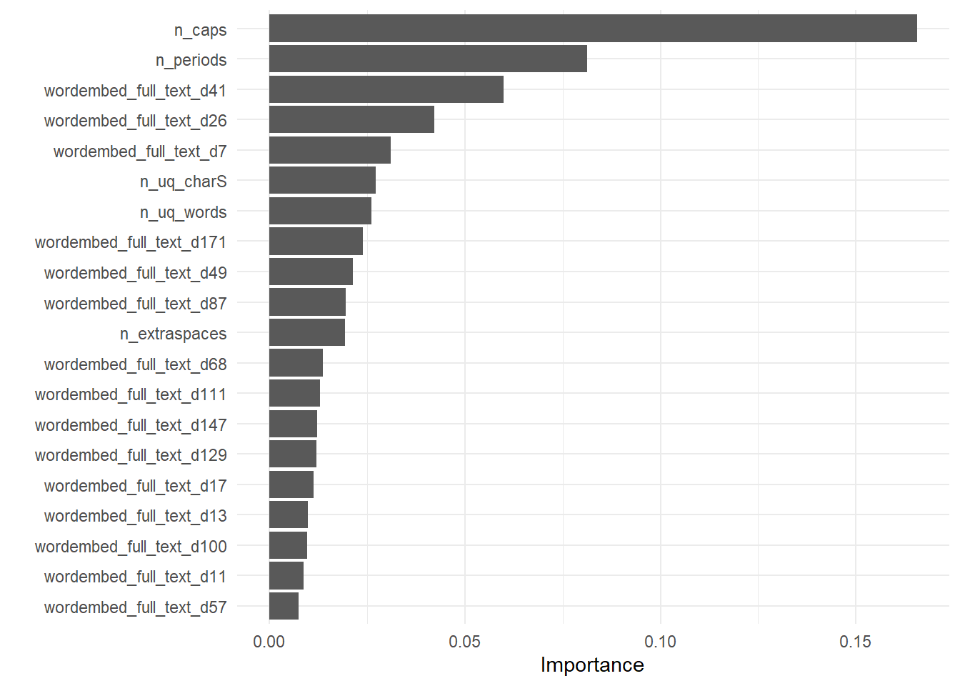

submission <- predict(
  classification_fit,
  
  submit_essays_raw |>
    bind_cols(predict(regression_fit, submit_essays_raw)) |>
    rename(regression_pred = .pred)
) |>
  transmute({{outcome}} := .pred_class) |>
  bind_cols(submission)

Warning in get_dtm(corp): dtm has 0 rows. Empty iterator?

Warning in get_dtm(corp): dtm has 0 rows. Empty iterator?

submission

Vocabulary

We fit for vocabulary first using an xgboost regression, using case weights to adjust for the frequency of occurrence of each value of vocabulary.

outcome <- outcomes[3]

regression_train_df <- train_essays_raw  |> 
                select(!!outcome, full_text) |> 
                case_weight_builder(outcome)

regression_wf <- workflow(recipe_builder(outcome = outcome), xgb_spec) |> 
       add_case_weights(case_wts)

folds <- vfold_cv(regression_train_df, strata = {{outcome}})

set.seed(42)  
rs <- fit_resamples(
  regression_wf,
  folds,
  control = control_resamples(save_pred = TRUE))

collect_metrics(rs) |> arrange(mean)

collect_predictions(rs) |> 
  plot_preds(.data[[outcome]]) +
  labs(y = "Predicted",
       title = paste0(outcome, " predictions against essays in held out folds"),
       subtitle = "The highest and lowest essays are not predicted well")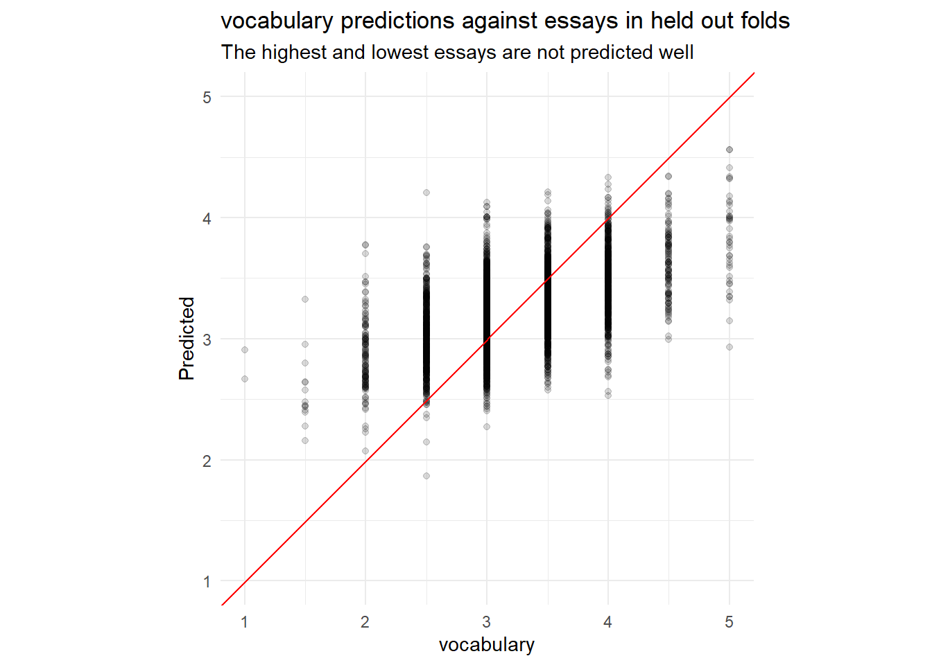

train_essays_raw[

collect_predictions(rs) |> 
  mutate(residual = .data[[outcome]] - .pred) |> 
  arrange(desc(abs(residual))) |> 
  slice_head(n = 5) |> 
  pull(.row)

, ] |> 
  select(full_text)

regression_fit <- parsnip::fit(regression_wf, 
                     regression_train_df)

Identifying examples with especially poor performance can help us follow up and investigate why these specific predictions are poor. Conceptually, its easy for a baseline know-nothing model to assign all essays to the median score of 3. The predictive power is in the ability to model the essays that are not 3 into buckets higher and lower than 3.

Because the ratings are a form of ordinal value, or even a likert scale, we will ensemble a second classification model that includes the output of the regression.

classification_train_df <- train_essays_raw  |> 
                select({{outcome}}, full_text) |> 
                bind_cols(
                  predict(
                    regression_fit,
                    regression_train_df
                  )
                ) |> 
               rename(regression_pred = .pred) |> 
               mutate({{outcome}} := factor(.data[[outcome]]))

classification_wf <- workflow(multiclass_recipe_builder(outcome = outcome), svm_spec) 

folds <- vfold_cv(classification_train_df, strata = !!outcome)

set.seed(42)  
rs <- fit_resamples(
  classification_wf,
  folds,
  metrics = metric_set(kap, accuracy),
  control = control_resamples(save_pred = TRUE))

collect_metrics(rs) |> arrange(mean)

collect_predictions(rs) |> 
  ggplot(aes(x = .data[[outcome]], y = abs(as.numeric(.data[[outcome]]) - as.numeric(.pred_class))/2)) +
  geom_violin() +
  scale_y_continuous(breaks = seq(-5,5,0.5)) +
  labs(y = "Residuals",
       title = "{{outcome}} Residual errors for essays in held out folds",
       subtitle = "The highest and lowest essays are still not predicted well")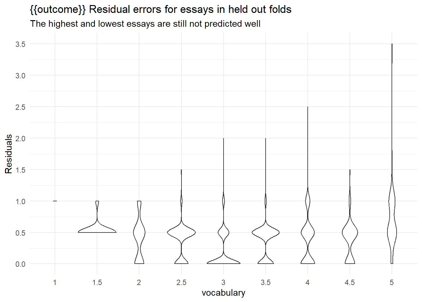

train_essays_raw[

collect_predictions(rs) |> 
  mutate(residual = as.numeric(.data[[outcome]]) - as.numeric(.pred_class)) |> 
  arrange(desc(abs(residual))) |> 
  slice_head(n = 5) |> 
  pull(.row)

, ] |> 
  select(full_text, {{outcome}})

collect_predictions(rs) |> 
  rmse(truth = as.numeric(.data[[outcome]])/2, estimate = as.numeric(.pred_class)/2)

Results here aren’t great, but they are more are less competitive with the leaderboard figures.

The final fitting ensembles both the regression and classification fits, and makes a prediction on the submission essays.

classification_fit <- parsnip::fit(classification_wf,
                                   classification_train_df)

extract_fit_engine(regression_fit) |> 
  vip::vip(num_features = 20)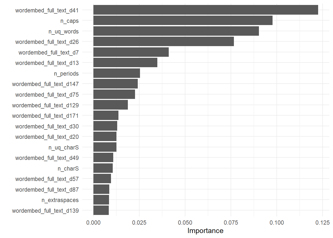

submission <- predict(
  classification_fit,
  
  submit_essays_raw |>
    bind_cols(predict(regression_fit, submit_essays_raw)) |>
    rename(regression_pred = .pred)
) |>
  transmute({{outcome}} := .pred_class) |>
  bind_cols(submission)

Warning in get_dtm(corp): dtm has 0 rows. Empty iterator?

Warning in get_dtm(corp): dtm has 0 rows. Empty iterator?

submission

Phraseology

We fit for phraseology first using an xgboost regression, using case weights to adjust for the frequency of occurrence of each value of phraseology.

outcome <- outcomes[4]

regression_train_df <- train_essays_raw  |> 
                select(!!outcome, full_text) |> 
                case_weight_builder(outcome)

regression_wf <- workflow(recipe_builder(outcome = outcome), xgb_spec) |> 
       add_case_weights(case_wts)

folds <- vfold_cv(regression_train_df, strata = {{outcome}})

set.seed(42)  
rs <- fit_resamples(
  regression_wf,
  folds,
  control = control_resamples(save_pred = TRUE))

collect_metrics(rs) |> arrange(mean)

collect_predictions(rs) |> 
  plot_preds(.data[[outcome]]) +
  labs(y = "Predicted",
       title = paste0(outcome, " predictions against essays in held out folds"),
       subtitle = "The highest and lowest essays are not predicted well")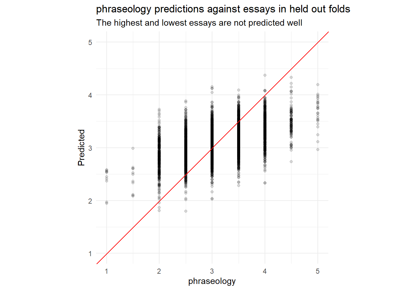

train_essays_raw[

collect_predictions(rs) |> 
  mutate(residual = .data[[outcome]] - .pred) |> 
  arrange(desc(abs(residual))) |> 
  slice_head(n = 5) |> 
  pull(.row)

, ] |> 
  select(full_text)

regression_fit <- parsnip::fit(regression_wf, 
                     regression_train_df)

Identifying examples with especially poor performance can help us follow up and investigate why these specific predictions are poor. Conceptually, its easy for a baseline know-nothing model to assign all essays to the median score of 3. The predictive power is in the ability to model the essays that are not 3 into buckets higher and lower than 3.

Because the ratings are a form of ordinal value, or even a likert scale, we will ensemble a second classification model that includes the output of the regression.

classification_train_df <- train_essays_raw  |> 
                select({{outcome}}, full_text) |> 
                bind_cols(
                  predict(
                    regression_fit,
                    regression_train_df
                  )
                ) |> 
               rename(regression_pred = .pred) |> 
               mutate({{outcome}} := factor(.data[[outcome]]))

classification_wf <- workflow(multiclass_recipe_builder(outcome = outcome), svm_spec) 

folds <- vfold_cv(classification_train_df, strata = !!outcome)

set.seed(42)  
rs <- fit_resamples(
  classification_wf,
  folds,
  metrics = metric_set(kap, accuracy),
  control = control_resamples(save_pred = TRUE))

collect_metrics(rs) |> arrange(mean)

collect_predictions(rs) |> 
  ggplot(aes(x = .data[[outcome]], y = abs(as.numeric(.data[[outcome]]) - as.numeric(.pred_class))/2)) +
  geom_violin() +
  scale_y_continuous(breaks = seq(-5,5,0.5)) +
  labs(y = "Residuals",
       title = "{{outcome}} Residual errors for essays in held out folds",
       subtitle = "The highest and lowest essays are still not predicted well")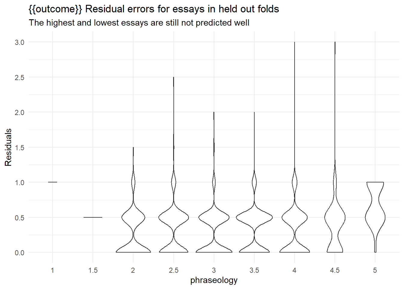

train_essays_raw[

collect_predictions(rs) |> 
  mutate(residual = as.numeric(.data[[outcome]]) - as.numeric(.pred_class)) |> 
  arrange(desc(abs(residual))) |> 
  slice_head(n = 5) |> 
  pull(.row)

, ] |> 
  select(full_text, {{outcome}})

collect_predictions(rs) |> 
  rmse(truth = as.numeric(.data[[outcome]])/2, estimate = as.numeric(.pred_class)/2)

Results here aren’t great, but they are more are less competitive with the leaderboard figures.

The final fitting ensembles both the regression and classification fits, and makes a prediction on the submission essays.

classification_fit <- parsnip::fit(classification_wf,
                                   classification_train_df)

extract_fit_engine(regression_fit) |> 
  vip::vip(num_features = 20)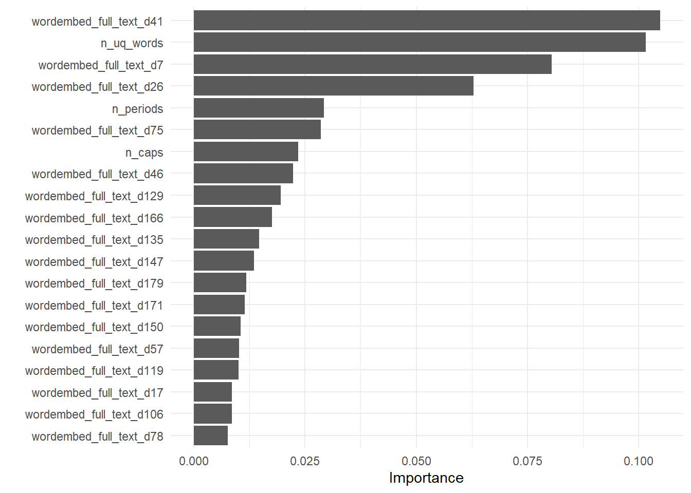

submission <- predict(
  classification_fit,
  
  submit_essays_raw |>
    bind_cols(predict(regression_fit, submit_essays_raw)) |>
    rename(regression_pred = .pred)
) |>
  transmute({{outcome}} := .pred_class) |>
  bind_cols(submission)

Warning in get_dtm(corp): dtm has 0 rows. Empty iterator?

Warning in get_dtm(corp): dtm has 0 rows. Empty iterator?

submission

Grammar

We fit for grammar first using an xgboost regression, using case weights to adjust for the frequency of occurrence of each value of grammar.

outcome <- outcomes[5]

regression_train_df <- train_essays_raw  |> 
                select(!!outcome, full_text) |> 
                case_weight_builder(outcome)

regression_wf <- workflow(recipe_builder(outcome = outcome), xgb_spec) |> 
       add_case_weights(case_wts)

folds <- vfold_cv(regression_train_df, strata = {{outcome}})

set.seed(42)  
rs <- fit_resamples(
  regression_wf,
  folds,
  control = control_resamples(save_pred = TRUE))

collect_metrics(rs) |> arrange(mean)

collect_predictions(rs) |> 
  plot_preds(.data[[outcome]]) +
  labs(y = "Predicted",
       title = paste0(outcome, " predictions against essays in held out folds"),
       subtitle = "The highest and lowest essays are not predicted well")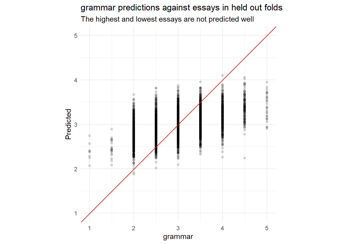

train_essays_raw[

collect_predictions(rs) |> 
  mutate(residual = .data[[outcome]] - .pred) |> 
  arrange(desc(abs(residual))) |> 
  slice_head(n = 5) |> 
  pull(.row)

, ] |> 
  select(full_text)

regression_fit <- parsnip::fit(regression_wf, 
                     regression_train_df)

Identifying examples with especially poor performance can help us follow up and investigate why these specific predictions are poor. Conceptually, its easy for a baseline know-nothing model to assign all essays to the median score of 3. The predictive power is in the ability to model the essays that are not 3 into buckets higher and lower than 3.

Because the ratings are a form of ordinal value, or even a likert scale, we will ensemble a second classification model that includes the output of the regression.

classification_train_df <- train_essays_raw  |> 
                select({{outcome}}, full_text) |> 
                bind_cols(
                  predict(
                    regression_fit,
                    regression_train_df
                  )
                ) |> 
               rename(regression_pred = .pred) |> 
               mutate({{outcome}} := factor(.data[[outcome]]))

classification_wf <- workflow(multiclass_recipe_builder(outcome = outcome), svm_spec) 

folds <- vfold_cv(classification_train_df, strata = !!outcome)

set.seed(42)  
rs <- fit_resamples(
  classification_wf,
  folds,
  metrics = metric_set(kap, accuracy),
  control = control_resamples(save_pred = TRUE))

collect_metrics(rs) |> arrange(mean)

collect_predictions(rs) |> 
  ggplot(aes(x = .data[[outcome]], y = abs(as.numeric(.data[[outcome]]) - as.numeric(.pred_class))/2)) +
  geom_violin() +
  scale_y_continuous(breaks = seq(-5,5,0.5)) +
  labs(y = "Residuals",
       title = "{{outcome}} Residual errors for essays in held out folds",
       subtitle = "The highest and lowest essays are still not predicted well")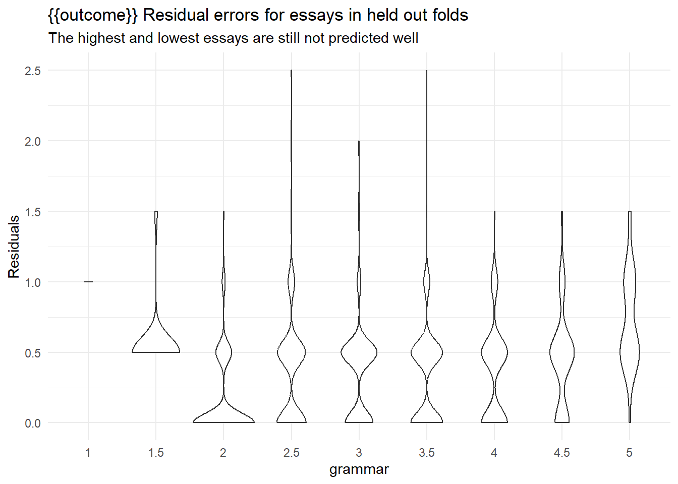

train_essays_raw[

collect_predictions(rs) |> 
  mutate(residual = as.numeric(.data[[outcome]]) - as.numeric(.pred_class)) |> 
  arrange(desc(abs(residual))) |> 
  slice_head(n = 5) |> 
  pull(.row)

, ] |> 
  select(full_text, {{outcome}})

collect_predictions(rs) |> 
  rmse(truth = as.numeric(.data[[outcome]])/2, estimate = as.numeric(.pred_class)/2)

Results here aren’t great, but they are more are less competitive with the leaderboard figures.

The final fitting ensembles both the regression and classification fits, and makes a prediction on the submission essays.

classification_fit <- parsnip::fit(classification_wf,
                                   classification_train_df)

extract_fit_engine(regression_fit) |> 
  vip::vip(num_features = 20)

submission <- predict(
  classification_fit,
  
  submit_essays_raw |>
    bind_cols(predict(regression_fit, submit_essays_raw)) |>
    rename(regression_pred = .pred)
) |>
  transmute({{outcome}} := .pred_class) |>
  bind_cols(submission)

Warning in get_dtm(corp): dtm has 0 rows. Empty iterator?

Warning in get_dtm(corp): dtm has 0 rows. Empty iterator?

submission

Conventions

We fit for conventions first using an xgboost regression, using case weights to adjust for the frequency of occurrence of each value of conventions.

outcome <- outcomes[6]

regression_train_df <- train_essays_raw  |> 
                select(!!outcome, full_text) |> 
                case_weight_builder(outcome)

regression_wf <- workflow(recipe_builder(outcome = outcome), xgb_spec) |> 
       add_case_weights(case_wts)

folds <- vfold_cv(regression_train_df, strata = {{outcome}})

set.seed(42)  
rs <- fit_resamples(
  regression_wf,
  folds,
  control = control_resamples(save_pred = TRUE))

collect_metrics(rs) |> arrange(mean)

collect_predictions(rs) |> 
  plot_preds(.data[[outcome]]) +
  labs(y = "Predicted",
       title = paste0(outcome, " predictions against essays in held out folds"),
       subtitle = "The highest and lowest essays are not predicted well")

train_essays_raw[

collect_predictions(rs) |> 
  mutate(residual = .data[[outcome]] - .pred) |> 
  arrange(desc(abs(residual))) |> 
  slice_head(n = 5) |> 
  pull(.row)

, ] |> 
  select(full_text)

regression_fit <- parsnip::fit(regression_wf, 
                     regression_train_df)

Identifying examples with especially poor performance can help us follow up and investigate why these specific predictions are poor. Conceptually, its easy for a baseline know-nothing model to assign all essays to the median score of 3. The predictive power is in the ability to model the essays that are not 3 into buckets higher and lower than 3.

Because the ratings are a form of ordinal value, or even a likert scale, we will ensemble a second classification model that includes the output of the regression.

classification_train_df <- train_essays_raw  |> 
                select({{outcome}}, full_text) |> 
                bind_cols(
                  predict(
                    regression_fit,
                    regression_train_df
                  )
                ) |> 
               rename(regression_pred = .pred) |> 
               mutate({{outcome}} := factor(.data[[outcome]]))

classification_wf <- workflow(multiclass_recipe_builder(outcome = outcome), svm_spec) 

folds <- vfold_cv(classification_train_df, strata = !!outcome)

set.seed(42)  
rs <- fit_resamples(
  classification_wf,
  folds,
  metrics = metric_set(kap, accuracy),
  control = control_resamples(save_pred = TRUE))

collect_metrics(rs) |> arrange(mean)

collect_predictions(rs) |> 
  ggplot(aes(x = .data[[outcome]], y = abs(as.numeric(.data[[outcome]]) - as.numeric(.pred_class))/2)) +
  geom_violin() +
  scale_y_continuous(breaks = seq(-5,5,0.5)) +
  labs(y = "Residuals",
       title = "{{outcome}} Residual errors for essays in held out folds",
       subtitle = "The highest and lowest essays are still not predicted well")

train_essays_raw[

collect_predictions(rs) |> 
  mutate(residual = as.numeric(.data[[outcome]]) - as.numeric(.pred_class)) |> 
  arrange(desc(abs(residual))) |> 
  slice_head(n = 5) |> 
  pull(.row)

, ] |> 
  select(full_text, {{outcome}})

collect_predictions(rs) |> 
  rmse(truth = as.numeric(.data[[outcome]])/2, estimate = as.numeric(.pred_class)/2)

Results here aren’t great, but they are more are less competitive with the leaderboard figures.

The final fitting ensembles both the regression and classification fits, and makes a prediction on the submission essays.

classification_fit <- parsnip::fit(classification_wf,
                                   classification_train_df)

extract_fit_engine(regression_fit) |> 
  vip::vip(num_features = 20)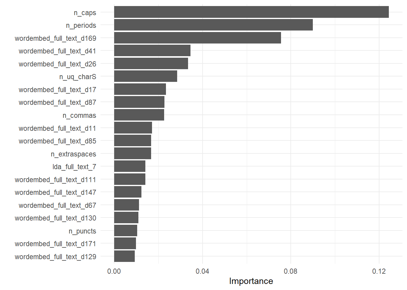

submission <- predict(
  classification_fit,
  
  submit_essays_raw |>
    bind_cols(predict(regression_fit, submit_essays_raw)) |>
    rename(regression_pred = .pred)
) |>
  transmute({{outcome}} := .pred_class) |>
  bind_cols(submission)

Warning in get_dtm(corp): dtm has 0 rows. Empty iterator?

Warning in get_dtm(corp): dtm has 0 rows. Empty iterator?

submission

The Submission

Kaggle’s system runs the workbook twice. The first time is on the tiny three line public test dataset here. The second time is on a much much larger hidden test dataset. As a check to simulate how the hidden datset might fit, we could re-fit on the train dataset text across all of the fits.

submission

# write_csv(submission, here::here("data", "submission.csv"))

Outcome

Not only was this exercise a good study of Likert evaluation data, but also of NLP techniques and of statistical resampling to assure that the model performs on unseen data. The resulting models here lack the predictive power needed for production use.

Session information

sessionInfo()

R version 4.2.2 (2022-10-31 ucrt)
Platform: x86_64-w64-mingw32/x64 (64-bit)
Running under: Windows 10 x64 (build 22621)

Matrix products: default

locale:
[1] LC_COLLATE=English_United States.utf8 
[2] LC_CTYPE=English_United States.utf8   
[3] LC_MONETARY=English_United States.utf8
[4] LC_NUMERIC=C                          
[5] LC_TIME=English_United States.utf8    

attached base packages:
[1] stats     graphics  grDevices utils     datasets  methods   base     

other attached packages:
 [1] LiblineaR_2.10-22  xgboost_1.6.0.1    textfeatures_0.3.3 textrecipes_1.0.1 
 [5] tidytext_0.3.4     text2vec_0.6.3     yardstick_1.1.0    workflowsets_1.0.0
 [9] workflows_1.1.2    tune_1.0.1         rsample_1.1.0      recipes_1.0.3     
[13] parsnip_1.0.3      modeldata_1.0.1    infer_1.0.4        dials_1.1.0       
[17] scales_1.2.1       broom_1.0.1        tidymodels_1.0.0   forcats_0.5.2     
[21] stringr_1.5.0      dplyr_1.0.10       purrr_0.3.5        readr_2.1.3       
[25] tidyr_1.2.1        tibble_3.1.8       ggplot2_3.4.0      tidyverse_1.3.2   
[29] workflowr_1.7.0   

loaded via a namespace (and not attached):
  [1] readxl_1.4.1           backports_1.4.1        splines_4.2.2         
  [4] listenv_0.8.0          SnowballC_0.7.0        tidylo_0.2.0          
  [7] digest_0.6.30          ca_0.71.1              foreach_1.5.2         
 [10] htmltools_0.5.3        float_0.3-0            fansi_1.0.3           
 [13] magrittr_2.0.3         memoise_2.0.1          googlesheets4_1.0.1   
 [16] tzdb_0.3.0             globals_0.16.2         modelr_0.1.10         
 [19] gower_1.0.0            vroom_1.6.0            hardhat_1.2.0         
 [22] timechange_0.1.1       colorspace_2.0-3       vip_0.3.2             
 [25] rappdirs_0.3.3         rvest_1.0.3            haven_2.5.1           
 [28] xfun_0.35              callr_3.7.3            crayon_1.5.2          
 [31] jsonlite_1.8.4         survival_3.4-0         iterators_1.0.14      
 [34] glue_1.6.2             registry_0.5-1         gtable_0.3.1          
 [37] gargle_1.2.1           ipred_0.9-13           future.apply_1.10.0   
 [40] mlapi_0.1.1            DBI_1.1.3              Rcpp_1.0.9            
 [43] GPfit_1.0-8            bit_4.0.5              lava_1.7.0            
 [46] prodlim_2019.11.13     httr_1.4.4             RColorBrewer_1.1-3    
 [49] ellipsis_0.3.2         farver_2.1.1           pkgconfig_2.0.3       
 [52] nnet_7.3-18            sass_0.4.4             dbplyr_2.2.1          
 [55] utf8_1.2.2             here_1.0.1             labeling_0.4.2        
 [58] tidyselect_1.2.0       rlang_1.0.6            DiceDesign_1.9        
 [61] later_1.3.0            munsell_0.5.0          cellranger_1.1.0      
 [64] tools_4.2.2            cachem_1.0.6           cli_3.4.1             
 [67] corrr_0.4.4            generics_0.1.3         rsparse_0.5.1         
 [70] evaluate_0.18          fastmap_1.1.0          yaml_2.3.6            
 [73] textdata_0.4.4         processx_3.8.0         RhpcBLASctl_0.21-247.1
 [76] knitr_1.41             bit64_4.0.5            fs_1.5.2              
 [79] lgr_0.4.4              future_1.29.0          whisker_0.4.1         
 [82] xml2_1.3.3             tokenizers_0.2.3       compiler_4.2.2        
 [85] rstudioapi_0.14        reprex_2.0.2           lhs_1.1.5             
 [88] bslib_0.4.1            stringi_1.7.8          highr_0.9             
 [91] ps_1.7.2               lattice_0.20-45        Matrix_1.5-3          
 [94] conflicted_1.1.0       vctrs_0.5.1            pillar_1.8.1          
 [97] lifecycle_1.0.3        furrr_0.3.1            jquerylib_0.1.4       
[100] data.table_1.14.6      seriation_1.4.0        httpuv_1.6.6          
[103] R6_2.5.1               TSP_1.2-1              promises_1.2.0.1      
[106] gridExtra_2.3          janeaustenr_1.0.0      parallelly_1.32.1     
[109] codetools_0.2-18       MASS_7.3-58.1          assertthat_0.2.1      
[112] rprojroot_2.0.3        withr_2.5.0            parallel_4.2.2        
[115] hms_1.1.2              grid_4.2.2             rpart_4.1.19          
[118] timeDate_4021.106      class_7.3-20           rmarkdown_2.18        
[121] googledrive_2.0.0      git2r_0.30.1           getPass_0.2-2         
[124] lubridate_1.9.0