Washington State Trails
Jim Gruman
November 27, 2020
Last updated: 2021-09-22
Checks: 7 0
Knit directory: myTidyTuesday/
This reproducible R Markdown analysis was created with workflowr (version 1.6.2). The Checks tab describes the reproducibility checks that were applied when the results were created. The Past versions tab lists the development history.
Great! Since the R Markdown file has been committed to the Git repository, you know the exact version of the code that produced these results.
Great job! The global environment was empty. Objects defined in the global environment can affect the analysis in your R Markdown file in unknown ways. For reproduciblity it’s best to always run the code in an empty environment.
The command set.seed(20210907) was run prior to running the code in the R Markdown file. Setting a seed ensures that any results that rely on randomness, e.g. subsampling or permutations, are reproducible.
Great job! Recording the operating system, R version, and package versions is critical for reproducibility.
Nice! There were no cached chunks for this analysis, so you can be confident that you successfully produced the results during this run.
Great job! Using relative paths to the files within your workflowr project makes it easier to run your code on other machines.
Great! You are using Git for version control. Tracking code development and connecting the code version to the results is critical for reproducibility.
The results in this page were generated with repository version 125b398. See the Past versions tab to see a history of the changes made to the R Markdown and HTML files.
Note that you need to be careful to ensure that all relevant files for the analysis have been committed to Git prior to generating the results (you can use wflow_publish or wflow_git_commit). workflowr only checks the R Markdown file, but you know if there are other scripts or data files that it depends on. Below is the status of the Git repository when the results were generated:
Ignored files:
    Ignored:    .Rhistory
    Ignored:    .Rproj.user/
    Ignored:    catboost_info/
    Ignored:    data/2021-09-08/
    Ignored:    data/acs_poverty.rds
    Ignored:    data/fmhpi.rds
    Ignored:    data/grainstocks.rds
    Ignored:    data/hike_data.rds
    Ignored:    data/us_states.rds
    Ignored:    data/us_states_hexgrid.geojson
    Ignored:    data/weatherstats_toronto_daily.csv

Untracked files:
    Untracked:  code/work list batch targets.R
    Untracked:  figure/
Note that any generated files, e.g. HTML, png, CSS, etc., are not included in this status report because it is ok for generated content to have uncommitted changes.
These are the previous versions of the repository in which changes were made to the R Markdown (analysis/WashingtonTrails.Rmd) and HTML (docs/WashingtonTrails.html) files. If you’ve configured a remote Git repository (see ?wflow_git_remote), click on the hyperlinks in the table below to view the files as they were in that past version.
| File | Version | Author | Date | Message |
|---|---|---|---|---|
| Rmd | 125b398 | opus1993 | 2021-09-22 | adopt stat_dots in trail lengths distribution chart |
| html | b30e599 | opus1993 | 2021-09-08 | Build site. |
| Rmd | 9484929 | opus1993 | 2021-09-08 | suppress package startup messages |
The data this week comes from Washington Trails Association courtesy of the TidyX crew, Ellis Hughes and Patrick Ward!
A video going through this data can be found on YouTube. Their original scraping code can be found on GitHub. The Washington Trails Assocation website includes this leaflet-style map visual
Let’s setup with the tidyverse, a theming package hrbrthemes, some web scraping tools, and table building tools.
suppressPackageStartupMessages({
library(tidyverse)
library(hrbrthemes)
extrafont::loadfonts(quiet = TRUE)
library(rvest)
library(gt)
library(fontawesome)
library(htmltools)

library(ggridges)

})

source(here::here("code","_common.R"),
       verbose = FALSE,
       local = knitr::knit_global())
Registered S3 method overwritten by 'tune':
method from
required_pkgs.model_spec parsnipggplot2::theme_set(theme_jim(base_size = 12))The original dataset provided by R4DS:
tt <- tidytuesdayR::tt_load("2020-11-24")
Downloading file 1 of 1: `hike_data.rds`After visiting the Washington Trails Association web site, I had expected to find 3869 hikes. It turns out that the R4DS scraping script skips all trails that lack elevation, gain, length, or rating figures. For more advanced visuals, I decided to go back and re-visit the scraping algorithm to also gather the geospatial coordinates in the sub pages. The update is here:
hike_data_rds <- here::here("data/hike_data.rds")

if (!file.exists(hike_data_rds)) {
  hike_pages <- 1:129

  hike_data <- lapply(hike_pages - 1, function(page) {
    start_int <- 30 * page

    page_url <- paste0(
      "https://www.wta.org/go-outside/hikes?b_start:int=",
      start_int
    )

    page_html <- read_html(page_url)

    page_html %>%
      html_nodes(".search-result-item") %>%
      map(
        function(hike) {
          hike_name <- hike %>%
            html_nodes(".item-header") %>%
            html_nodes(".listitem-title") %>%
            html_nodes("span") %>%
            html_text()

          hike_page <- hike %>%
            html_nodes(".item-header") %>%
            html_nodes(".listitem-title") %>%
            html_attr("href")

          hike_location <- hike %>%
            html_nodes(".item-header") %>%
            html_nodes(".region") %>%
            html_text()

          hike_desc <- hike %>%
            html_nodes(".hike-detail") %>%
            html_nodes(".listing-summary") %>%
            html_text() %>%
            stringr::str_trim(side = "both")

          hike_features <- hike %>%
            html_nodes(".hike-detail") %>%
            html_nodes(".trip-features") %>%
            html_nodes("img") %>%
            html_attr("title") %>%
            list()

          tibble(
            name = hike_name,
            location = hike_location,
            features = hike_features,
            description = hike_desc,
            hike_page = hike_page
          )
        }
      ) %>%
      bind_rows() %>%
      mutate(stats = map(hike_page, function(hike_page) {
        print(hike_page)

        stats_html <- read_html(hike_page)

        length <- stats_html %>%
          html_nodes(".hike-stat") %>%
          html_nodes("#distance") %>%
          html_nodes("span") %>%
          html_text()

        elevation <- stats_html %>%
          html_nodes(".hike-stat") %>%
          `[[`(3)

        elevation_state <- case_when(
          sum(html_text(elevation) %>% str_detect(c("Gain", "Point"))) == 2 ~ "both",
          html_text(elevation) %>% str_detect("Gain") ~ "gain",
          html_text(elevation) %>% str_detect("Point") ~ "highpoint",
          TRUE ~ "neither"
        )

        if (elevation_state == "both") {
          gain <- elevation %>%
            html_nodes("span") %>%
            html_text() %>%
            `[[`(1)

          highpoint <- elevation %>%
            html_nodes("span") %>%
            html_text() %>%
            `[[`(2)
        } else if (elevation_state == "highpoint") {
          highpoint <- elevation %>%
            html_nodes("span") %>%
            html_text()

          gain <- NA_character_
        } else if (elevation_state == "gain") {
          gain <- elevation %>%
            html_nodes("span") %>%
            html_text()

          highpoint <- NA_character_
        } else if (elevation_state == "neither") {
          highpoint <- NA_character_
          gain <- NA_character_
        }

        rating <- stats_html %>%
          html_nodes(".hike-stat") %>%
          `[[`(4) %>%
          html_nodes(".current-rating") %>%
          html_text()

        longitude <- if (is_empty(stats_html %>%
          html_nodes(".latlong") %>%
          html_node("span") %>%
          html_text())) {
          NA_character_
        } else {
          stats_html %>%
            html_nodes(".latlong") %>%
            html_nodes("span") %>%
            html_text() %>%
            `[[`(1)
        }

        latitude <- if (is_empty(stats_html %>%
          html_nodes(".latlong") %>%
          html_node("span") %>%
          html_text())) {
          NA_character_
        } else {
          stats_html %>%
            html_nodes(".latlong") %>%
            html_nodes("span") %>%
            html_text() %>%
            `[[`(2)
        }

        stats <- tibble(
          length = length,
          gain = gain,
          highpoint = highpoint,
          rating = rating,
          longitude = longitude,
          latitude = latitude
        )

        return(stats)
      }))
  }) %>%
    bind_rows() %>%
    unnest_wider(stats)

  hike_data <- hike_data %>%
    mutate(
      trip = case_when(
        grepl("roundtrip", length) ~ "roundtrip",
        grepl("one-way", length) ~ "one-way",
        grepl("of trails", length) ~ "trails"
      ),
      length_total = as.numeric(gsub("(\\d+[.]\\d+).*", "\\1", length)) * ((trip == "one-way") + 1)
    ) %>%
    mutate(
      across(c(length, gain, highpoint, longitude, latitude, rating), parse_number)
    )
  write_rds(hike_data, file = hike_data_rds)
} else {
  hike_data <- read_rds(hike_data_rds)
}
We will further separate the location field into region and subregion, by the hyphen.
hike_data <- hike_data %>%
  separate(location, into = c("region", "subregion"), sep = " -- ", fill = "right") %>%
  replace_na(list(subregion = "Other")) %>%
  mutate(across(c(name, region, subregion), as_factor))
First, a table of summarized trail data by Region
rating_stars <- function(rating, max_rating = 5) {
  rounded_rating <- floor(rating + 0.5)
  stars <- lapply(seq_len(max_rating), function(i) {
    if (i <= rounded_rating) {
      fontawesome::fa("star", fill = "orange")
    } else {
      fontawesome::fa("star", fill = "grey")
    }
  })
  label <- sprintf("%s out of %s", rating, max_rating)
  div_out <- div(title = label, "aria-label" = label, role = "img", stars)

  as.character(div_out) %>%
    gt::html()
}

hike_data %>%
  group_by(region, subregion) %>%
  summarize(
    total_length = round(sum(length, na.rm = TRUE)),
    average_gain = round(mean(gain, na.rm = TRUE)),
    min_rating = round(min(rating, na.rm = TRUE), 1),
    max_rating = round(max(rating, na.rm = TRUE), 1),
    number = n(),
    .groups = "drop"
  ) %>%
  mutate(
    subregion = fct_reorder(subregion, desc(number)),
    min_rating = map(min_rating, rating_stars),
    max_rating = map(max_rating, rating_stars)
  ) %>%
  select(region, subregion, number, total_length, average_gain, min_rating, max_rating) %>%
  arrange(region, subregion) %>%
  group_by(region) %>%
  gt() %>%
  tab_header(title = gt::html("<span style='color:darkgreen'>Washington State Hiking Trail Summary by Region</span>")) %>%
  cols_label(
    subregion = "Region",
    number = "Number of Trails",
    total_length = md("Total Milage All Trails"),
    average_gain = md("Average Elevation Gain (Feet)"),
    min_rating = md("**Min Rating**"),
    max_rating = md("**Max Rating**")
  ) %>%
  opt_row_striping() %>%
tab_options(data_row.padding = px(3))| Washington State Hiking Trail Summary by Region | |||||
|---|---|---|---|---|---|
| Region | Number of Trails | Total Milage All Trails | Average Elevation Gain (Feet) | Min Rating | Max Rating |
| North Cascades | |||||
| North Cascades Highway - Hwy 20 | 149 | 1272 | 2902 | ||
| Mountain Loop Highway | 147 | 907 | 2069 | ||
| Methow/Sawtooth | 92 | 550 | 2425 | ||
| Pasayten | 86 | 927 | 3008 | ||
| Mount Baker Area | 77 | 421 | 1756 | ||
| Other | 139 | 117 | 3754 | ||
| Mount Rainier Area | |||||
| Chinook Pass - Hwy 410 | 84 | 547 | 1611 | ||
| SW - Longmire/Paradise | 75 | 484 | 1810 | ||
| NW - Carbon River/Mowich | 39 | 411 | 2582 | ||
| NE - Sunrise/White River | 31 | 235 | 2402 | ||
| SE - Cayuse Pass/Stevens Canyon | 29 | 184 | 1567 | ||
| Other | 25 | 110 | 9300 | ||
| Southwest Washington | |||||
| Columbia River Gorge - WA | 62 | 460 | 1618 | ||
| Lewis River Region | 38 | 269 | 1115 | ||
| Vancouver Area | 34 | 112 | 109 | ||
| Columbia River Gorge - OR | 34 | 134 | 1231 | ||
| Long Beach Area | 24 | 73 | 147 | ||
| Other | 1 | 2 | NaN | ||
| Puget Sound and Islands | |||||
| Seattle-Tacoma Area | 266 | 902 | 273 | ||
| Bellingham Area | 89 | 378 | 662 | ||
| San Juan Islands | 47 | 142 | 543 | ||
| Whidbey Island | 33 | 157 | 356 | ||
| Other | 15 | 1242 | 120 | ||
| Olympic Peninsula | |||||
| Hood Canal | 111 | 781 | 2206 | ||
| Northern Coast | 104 | 707 | 1967 | ||
| Olympia | 60 | 282 | 696 | ||
| Pacific Coast | 56 | 417 | 928 | ||
| Kitsap Peninsula | 28 | 103 | 332 | ||
| Other | 12 | 24 | 2250 | ||
| Central Cascades | |||||
| Stevens Pass - West | 119 | 536 | 1638 | ||
| Stevens Pass - East | 96 | 798 | 2981 | ||
| Entiat Mountains/Lake Chelan | 95 | 695 | 2516 | ||
| Leavenworth Area | 70 | 389 | 2599 | ||
| Blewett Pass | 38 | 149 | 1171 | ||
| Other | 94 | 54 | 4238 | ||
| Snoqualmie Region | |||||
| Snoqualmie Pass | 123 | 814 | 2330 | ||
| Salmon La Sac/Teanaway | 122 | 723 | 2318 | ||
| North Bend Area | 107 | 655 | 2014 | ||
| Cle Elum Area | 26 | 168 | 1986 | ||
| Other | 21 | 24 | 3018 | ||
| South Cascades | |||||
| Mount St. Helens | 63 | 474 | 1548 | ||
| Mount Adams Area | 62 | 357 | 1324 | ||
| White Pass/Cowlitz River Valley | 62 | 501 | 1894 | ||
| Goat Rocks | 33 | 314 | 2018 | ||
| Dark Divide | 24 | 146 | 1536 | ||
| Other | 107 | 318 | 2322 | ||
| Central Washington | |||||
| Yakima | 59 | 368 | 1221 | ||
| Tri-Cities | 28 | 148 | 528 | ||
| Wenatchee | 28 | 124 | 935 | ||
| Potholes Region | 23 | 85 | 315 | ||
| Other | 2 | 1 | 30 | ||
| Grand Coulee | 13 | 54 | 363 | ||
| Eastern Washington | |||||
| Spokane Area/Coeur d'Alene | 108 | 638 | 831 | ||
| Okanogan Highlands/Kettle River Range | 54 | 412 | 1642 | ||
| Palouse and Blue Mountains | 54 | 548 | 1914 | ||
| Selkirk Range | 50 | 290 | 1580 | ||
| Other | 29 | 46 | 825 | ||
| Issaquah Alps | |||||
| Tiger Mountain | 60 | 245 | 1297 | ||
| Cougar Mountain | 55 | 89 | 397 | ||
| Squak Mountain | 25 | 82 | 1424 | ||
| Other | 21 | 82 | 320 | ||
| Taylor Mountain | 12 | 34 | 475 | ||
Another table, adapted from Kaustav Sen’s post
thumbs_up <- function(value) {
icon <- fa("thumbs-up", fill = "#38A605")
div(icon) %>%
as.character() %>%
html()
}
bar_chart <- function(value, color = "#DFB37D") {
glue::glue(
"<span style=\"display: inline-block;
direction: ltr; border-radius: 4px;
padding-right: 2px; background-color: {color};
color: {color}; width: {value}%\"> </span>"
) %>%
as.character() %>%
gt::html()
}
hike_data %>%
group_by(region) %>%
arrange(desc(rating)) %>%
slice(1:4) %>%
ungroup() %>%
select(
-description, -gain, -highpoint, -latitude, -longitude,
-hike_page, -subregion, -length_total, -trip
) %>%
mutate(
rating = if_else(is.na(rating), 0, rating),
length_bar = map(length, bar_chart),
rating = map(rating, rating_stars),
feature_present = 1,
feature_present = map(feature_present, thumbs_up)
) %>%
unnest_longer(features) %>%
mutate(features = str_replace(features, pattern = "/.+", replacement = "")) %>%
pivot_wider(
names_from = features,
values_from = feature_present
) %>%
group_by(region) %>%
arrange(-length) %>%
select(name, length, length_bar, rating, everything()) %>%
gt() %>%
cols_width(
"name" ~ px(250),
"length" ~ px(75),
"length_bar" ~ px(140),
"rating" ~ px(140),
4:last_col() ~ px(120)
) %>%
tab_spanner(
label = "Features",
columns = 5:last_col()
) %>%
cols_label(
name = "",
length = md("Length<br/>(in miles)"),
length_bar = "",
rating = "Rating"
) %>%
tab_header(
title = "Top Hiking Trails to visit in Washington",
subtitle = "The 4 top rated trails in each of the 11 major regions of Washington State"
) %>%
tab_source_note(
source_note = md("**Data:** Washington Trails Association | **Table:** Jim Gruman")
) %>%
tab_style(
style = cell_text(
font = google_font("Alegreya Sans SC"),
weight = "bold"
),
locations = list(cells_row_groups(), cells_column_spanners("Features"))
) %>%
tab_style(
style = cell_fill(
color = "#DFB37D",
alpha = 0.5
),
locations = cells_row_groups()
) %>%
tab_style(
style = cell_text(
font = google_font("Alegreya Sans"),
v_align = "bottom",
align = "center"
),
locations = cells_column_labels(columns = everything())
) %>%
tab_style(
style = cell_text(
font = google_font("Alegreya Sans"),
),
locations = cells_body("name")
) %>%
tab_style(
style = cell_text(
font = google_font("Alegreya Sans"),
align = "left",
size = px(30)
),
locations = cells_title("subtitle")
) %>%
tab_style(
style = cell_text(
size = "medium"
),
locations = cells_body(columns = 4:last_col())
) %>%
tab_style(
style = cell_text(
align = "left"
),
locations = cells_body(columns = "length_bar")
) %>%
tab_style(
style = cell_text(
font = google_font("Alegreya Sans SC"),
align = "left",
weight = "bold",
size = px(50)
),
locations = cells_title("title")
) %>%
opt_table_font(font = google_font("Fira Mono")) %>%
tab_options(
table.border.top.color = "white",
)| Top Hiking Trails to visit in Washington | |||||||||||||||||||
|---|---|---|---|---|---|---|---|---|---|---|---|---|---|---|---|---|---|---|---|
| The 4 top rated trails in each of the 11 major regions of Washington State | |||||||||||||||||||
| Length (in miles) |
Rating | Features | |||||||||||||||||
| Wildflowers | Ridges | Wildlife | Mountain views | Summits | Dogs allowed on leash | Fall foliage | Rivers | Lakes | NA | Dogs not allowed | Established campsites | Old growth | Good for kids | Waterfalls | Coast | ||||
| Central Cascades | |||||||||||||||||||
| Icicle Divide: Stevens Pass to Fourth of July | 45.00 | ||||||||||||||||||
| Little Annapurna | 7.30 | ||||||||||||||||||
| Blackbird Island - Waterfront Park | 2.00 | ||||||||||||||||||
| Bygone Byways Interpretive Trail | 1.00 | ||||||||||||||||||
| Eastern Washington | |||||||||||||||||||
| Kettle Crest Trail | 44.00 | ||||||||||||||||||
| Liberty Lake Regional Park - Liberty Lake Loop Trail | 8.40 | ||||||||||||||||||
| Wenatchee Guard Station | 5.80 | ||||||||||||||||||
| Columbia Mountain | 5.40 | ||||||||||||||||||
| Mount Rainier Area | |||||||||||||||||||
| Eastside Loop | 36.00 | ||||||||||||||||||
| Indian Bar - Summerland Traverse | 34.00 | ||||||||||||||||||
| Wonderland Trail - Mowich Lake to Sunrise via Spray Park | 20.50 | ||||||||||||||||||
| Old Mine Trail | 3.40 | ||||||||||||||||||
| North Cascades | |||||||||||||||||||
| Seven Pass Loop (Pasayten) | 26.60 | ||||||||||||||||||
| Glacier Peak Meadows | 25.00 | ||||||||||||||||||
| North Lake | 10.60 | ||||||||||||||||||
| Eldorado Peak | 10.00 | ||||||||||||||||||
| Olympic Peninsula | |||||||||||||||||||
| Capitol State Forest - McKenny Trail | 13.80 | ||||||||||||||||||
| Lyre Conservation Area | 2.50 | ||||||||||||||||||
| High Ridge Trail | 0.80 | ||||||||||||||||||
| Illahee State Park | 0.50 | ||||||||||||||||||
| Snoqualmie Region | |||||||||||||||||||
| Esmeralda Peak Loop | 12.10 | ||||||||||||||||||
| Mount Stuart | 11.10 | ||||||||||||||||||
| Tanner Landing Park | 1.00 | ||||||||||||||||||
| Roaring Creek | 0.60 | ||||||||||||||||||
| Central Washington | |||||||||||||||||||
| Ahtanum State Forest - Whites Ridge | 10.90 | ||||||||||||||||||
| Candy Mountain Trail | 3.60 | ||||||||||||||||||
| East Rim Waterworks Canyon | 3.00 | ||||||||||||||||||
| Ohme Gardens County Park | 1.00 | ||||||||||||||||||
| South Cascades | |||||||||||||||||||
| Plains of Abraham - Windy Pass Loop | 9.00 | ||||||||||||||||||
| Fossil Trail | 8.00 | ||||||||||||||||||
| Mountain Climbers Trail | 6.80 | ||||||||||||||||||
| Bench Lake Loop | 3.40 | ||||||||||||||||||
| Southwest Washington | |||||||||||||||||||
| Lewis and Clark Discovery Trail | 7.00 | ||||||||||||||||||
| Cussed Hollow | 5.00 | ||||||||||||||||||
| La Center Bottoms | 0.66 | ||||||||||||||||||
| Cape Disappointment State Park - Cape Disappointment Lighthouse | 0.60 | ||||||||||||||||||
| Puget Sound and Islands | |||||||||||||||||||
| Turtleback Mountain Preserve: Turtlehead Summit | 5.70 | ||||||||||||||||||
| Mount Grant Preserve | 4.60 | ||||||||||||||||||
| Leque Island - Stanwood Levee Trail | 1.40 | ||||||||||||||||||
| Nathan Chapman Memorial Trail | 0.60 | ||||||||||||||||||
| Issaquah Alps | |||||||||||||||||||
| Coyote Creek | 1.10 | ||||||||||||||||||
| Paw Print Connector | 1.10 | ||||||||||||||||||
| Nike Horse Trail | 0.60 | ||||||||||||||||||
| Long View Peak | 0.30 | ||||||||||||||||||
| Data: Washington Trails Association | Table: Jim Gruman | |||||||||||||||||||
What is the distribution of hiking trail lengths around the state regions?
Let’s build a helper function to add sample counts to categorical charts.
withfreq <- function(x) {
  tibble(x) %>%
    add_count(x) %>%
    mutate(combined = glue::glue("{ str_wrap(x, width = 20) } ({ n })")) %>%
    pull(combined)
}
hike_data %>%
filter(!is.na(length)) %>%
mutate(region = withfreq(region)) %>%
ggplot(aes(length, region, color = region)) +
ggdist::stat_dots(
## orientation to the left
side = "top",
## move geom up
justification = 0.1,
## adjust grouping (binning) of observations
binwidth = 0.02,
show.legend = FALSE
) +
geom_text(
data = . %>% filter(length > 150),
aes(label = stringr::str_wrap(name, 12)),
check_overlap = TRUE,
nudge_y = 0.4,
show.legend = FALSE
) +
# geom_density_ridges(alpha = 0.9, show.legend = FALSE) +
scale_x_log10(labels = scales::comma_format(accuracy = 1)) +
coord_cartesian(clip = "off") +
labs(
x = "Trail Lengths in Miles", y = NULL,
title = "Trail Lengths Available by Region",
subtitle = "(Counts of trails) SW Washington and the Cascades have more of the Longer Trails",
caption = "@jim_gruman | Data: TidyX"
) +
theme(panel.grid.major.y = element_blank())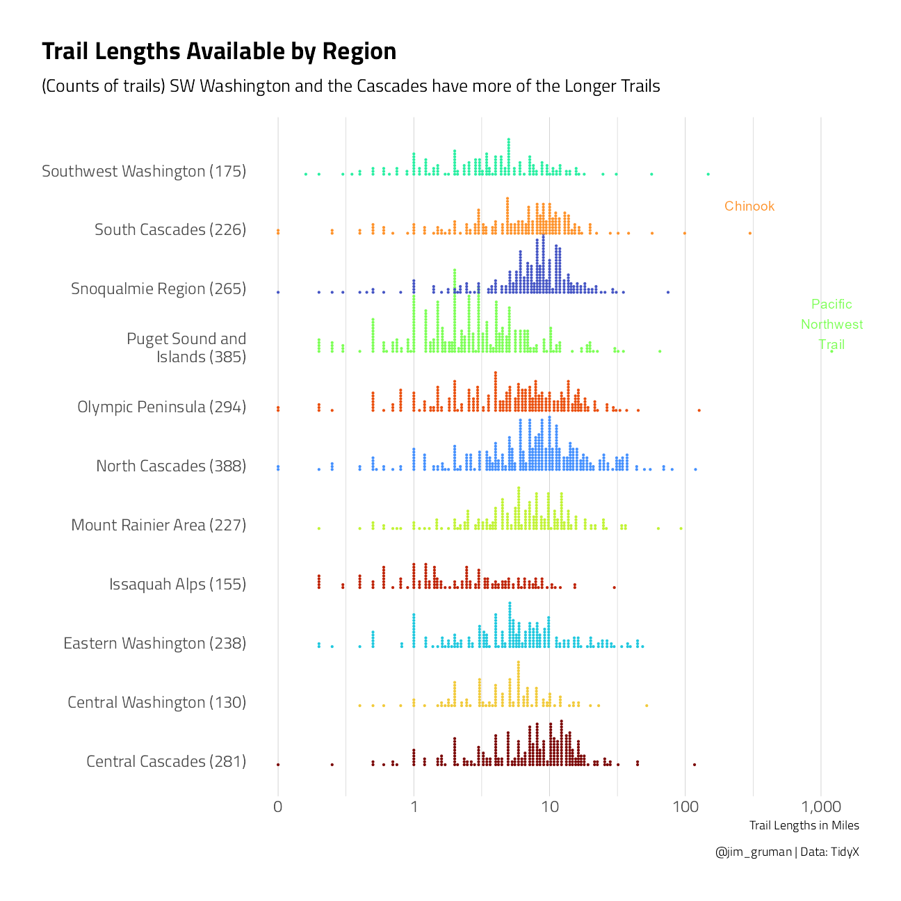
Let’s take a closer look at the features of each trail and the relationship with length:
hikes_complete <- hike_data %>%
  filter(length > 0.1) %>%
  mutate(
    hikeID = row_number(),
    length = log10(length),
    length = length %/% 0.2 * 0.2
  ) %>%
  select(hikeID, length, features) %>%
  unnest(features) %>%
  count(length, features) %>%
  complete(length, features, fill = list(n = 0)) %>%
  group_by(length) %>%
  mutate(length_total = sum(n)) %>%
  ungroup()

hikes_complete
# A tibble: 240 x 4
length features n length_total
<dbl> <chr> <dbl> <dbl>
1 -0.8 Coast 3 104
2 -0.8 Dogs allowed on leash 18 104
3 -0.8 Dogs not allowed 3 104
4 -0.8 Established campsites 0 104
5 -0.8 Fall foliage 8 104
6 -0.8 Good for kids 29 104
7 -0.8 Lakes 4 104
8 -0.8 Mountain views 7 104
9 -0.8 Old growth 4 104
10 -0.8 Ridges/passes 2 104
# ... with 230 more rowsslopes <- hikes_complete %>%
nest_by(features) %>%
mutate(model = list(glm(cbind(n, length_total) ~ length,
family = "binomial",
data = data
))) %>%
summarize(broom::tidy(model)) %>%
ungroup() %>%
filter(term == "length") %>%
mutate(p.value = p.adjust(p.value)) %>%
filter(p.value < 0.05) %>%
arrange(estimate)hikes_complete %>%
mutate(length_percent = n / length_total) %>%
inner_join(slopes) %>%
mutate(features = fct_reorder(features, -estimate)) %>%
ggplot(aes(length, length_percent)) +
geom_smooth(method = "lm") +
geom_point() +
facet_wrap(~features) +
scale_y_continuous(labels = scales::percent_format(accuracy = 1)) +
labs(
x = "Length of each trail (log10 scale)",
y = "% of trails with each feature",
title = "Which features of Washington hikes are associated with longer trails?",
caption = "@jim_gruman | Data: TidyX"
)
sessionInfo()R version 4.1.1 (2021-08-10)
Platform: x86_64-w64-mingw32/x64 (64-bit)
Running under: Windows 10 x64 (build 19043)
Matrix products: default
locale:
[1] LC_COLLATE=English_United States.1252
[2] LC_CTYPE=English_United States.1252
[3] LC_MONETARY=English_United States.1252
[4] LC_NUMERIC=C
[5] LC_TIME=English_United States.1252
attached base packages:
[1] stats graphics grDevices utils datasets methods base
other attached packages:
[1] ggridges_0.5.3 htmltools_0.5.2 fontawesome_0.2.2 gt_0.3.1
[5] rvest_1.0.1 hrbrthemes_0.8.0 forcats_0.5.1 stringr_1.4.0
[9] dplyr_1.0.7 purrr_0.3.4 readr_2.0.1 tidyr_1.1.3
[13] tibble_3.1.4 ggplot2_3.3.5 tidyverse_1.3.1 workflowr_1.6.2
loaded via a namespace (and not attached):
[1] readxl_1.3.1 backports_1.2.1 systemfonts_1.0.2
[4] workflows_0.2.3 selectr_0.4-2 plyr_1.8.6
[7] tidytuesdayR_1.0.1 splines_4.1.1 listenv_0.8.0
[10] usethis_2.0.1 digest_0.6.27 foreach_1.5.1
[13] yardstick_0.0.8 viridis_0.6.1 parsnip_0.1.7.900
[16] fansi_0.5.0 checkmate_2.0.0 magrittr_2.0.1
[19] tune_0.1.6 tzdb_0.1.2 recipes_0.1.16
[22] globals_0.14.0 modelr_0.1.8 gower_0.2.2
[25] extrafont_0.17 R.utils_2.10.1 extrafontdb_1.0
[28] hardhat_0.1.6 rsample_0.1.0 dials_0.0.10
[31] colorspace_2.0-2 ggdist_3.0.0 textshaping_0.3.5
[34] haven_2.4.3 xfun_0.26 crayon_1.4.1
[37] jsonlite_1.7.2 survival_3.2-11 iterators_1.0.13
[40] glue_1.4.2 gtable_0.3.0 ipred_0.9-12
[43] distributional_0.2.2 R.cache_0.15.0 Rttf2pt1_1.3.9
[46] future.apply_1.8.1 scales_1.1.1 infer_1.0.0
[49] DBI_1.1.1 Rcpp_1.0.7 viridisLite_0.4.0
[52] GPfit_1.0-8 lava_1.6.10 prodlim_2019.11.13
[55] httr_1.4.2 ellipsis_0.3.2 farver_2.1.0
[58] pkgconfig_2.0.3 R.methodsS3_1.8.1 nnet_7.3-16
[61] sass_0.4.0 dbplyr_2.1.1 utf8_1.2.2
[64] here_1.0.1 labeling_0.4.2 tidyselect_1.1.1
[67] rlang_0.4.11 DiceDesign_1.9 later_1.3.0
[70] munsell_0.5.0 cellranger_1.1.0 tools_4.1.1
[73] cachem_1.0.6 cli_3.0.1 generics_0.1.0
[76] broom_0.7.9 evaluate_0.14 fastmap_1.1.0
[79] yaml_2.2.1 ragg_1.1.3 rematch2_2.1.2
[82] knitr_1.34 fs_1.5.0 nlme_3.1-152
[85] future_1.22.1 whisker_0.4 R.oo_1.24.0
[88] xml2_1.3.2 compiler_4.1.1 rstudioapi_0.13
[91] curl_4.3.2 reprex_2.0.1 lhs_1.1.3
[94] bslib_0.3.0 stringi_1.7.4 highr_0.9
[97] gdtools_0.2.3 lattice_0.20-44 Matrix_1.3-4
[100] commonmark_1.7 styler_1.6.1 conflicted_1.0.4
[103] vctrs_0.3.8 tidymodels_0.1.3 pillar_1.6.2
[106] lifecycle_1.0.0 furrr_0.2.3 jquerylib_0.1.4
[109] httpuv_1.6.3 R6_2.5.1 promises_1.2.0.1
[112] gridExtra_2.3 parallelly_1.28.1 codetools_0.2-18
[115] MASS_7.3-54 assertthat_0.2.1 rprojroot_2.0.2
[118] withr_2.4.2 mgcv_1.8-36 parallel_4.1.1
[121] hms_1.1.0 grid_4.1.1 rpart_4.1-15
[124] timeDate_3043.102 class_7.3-19 rmarkdown_2.11
[127] git2r_0.28.0 pROC_1.18.0 lubridate_1.7.10